
Analysis of Chutes and Ladders
Have you ever played the game Chutes and Ladders®?
 |
In England, where I grew up, it goes by the name Snakes and Ladders. According to the internet, it is possible to trace the origins of the game back to the 2nd Century B.C. as the Indian game of Paramapada Sopanam — "The Ladder to Salvation." |
It was invented by Hindu spiritual leaders to teach children about the rewards of good deeds and the negative consequences of bad ones. The snakes represent vices and poor decisions, and the ladders represent virtues and sound morality. The game first made its way to England in 1892, and was commercially sold in the United States in 1943 by Milton Bradley under the name Chutes and Ladders. It has been speculated that Square 100 represents the Hindu idea of Nirvana (and you thought it was just a kids’ game!)
Gameplay
|
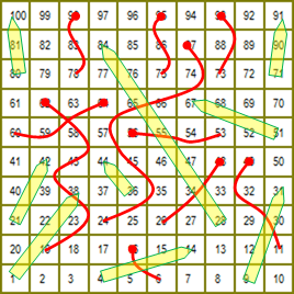
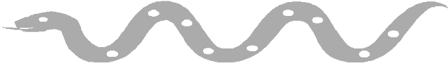
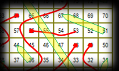
The game is played on a 10x10 gridded board which is numbered, sequentially, in a zig-zag pattern from 1 (the start), in the lower left corner, to 100 (the end), in the top left corner. At various locations on the board are placed snakes and ladders, each of which connects a pair of squares. A representation of the board that our family plays on is shown to the right. (Snakes are shown in red with a dot representing their heads, and ladders in light green with a point showing the direction of travel). All players start off the board, and roll a single die (or in the case of the Milton Bradley version, flick a spinner labeled 1 through 6), moving the corresponding number of squares. If the completion of your move results in your token landing at the foot of a ladder, you instantly climb to the top of that ladder. Correspondingly, if your move lands you on the head of a snake, you are forced to slide down the snake to an earlier square. There are no consequences to landing on the top of a ladder or the tail of a snake. These snakes/ladders are one-way events (Mathematically, we described this as a Directed Graph ). The first player to square 100 wins. |
|
The official rules of the Milton Bradley variant of game state that, to win, you must land exactly on square 100 (staying put and missing your turn if your roll would overshoot). Our (impatient) family hates this rule with a passion and so we elect to ignore it! (as we do on all similar games that dictate ”exact roll needed to finish”)
All the mathematical analysis in this blog follows our house rule — If you make it to, or past, the finish square, you win!
How long does an average game take?
|
Because of the cyclic nature of the game (landing on a snake can send you backwards and, if you are incredibly unlucky, you can land on another, and another …), there is no theoretical upper bound to the number of moves a game can take. Thankfully, however, the probability for long duration games rapidly asymptotes to insignificance. In the analysis that will be described below, a billion games of Chutes and Ladders were played, and the longest recorded game took 394 moves. 97.6% of games (thankfully) take 100 moves or less to complete. But we’re getting ahead of ourselves … |
 |
An Objectivist and Bayesian walk into a bar …
If we have a system (game, machine, coin-flip, action …) that we wish to calculate the probability of some event about (winning, losing, length of game …) we have two basic mechanism to calculate these probabilities:
– Experimentation (Objectivizing)
– Formal Modeling (Subjectivizing – also called a Bayesian approach).
These are big words, but the concepts are really simple.
Objective Approach
In an objective approach, you simply repeat an experiment many times and record the relative frequency of the results; More likely events happen more often, less likely events less often. Proportionally, the results advise you of the relative probabilities. The more samples or experiments you run, the higher the confidence you have in your results.
 |
If you wanted to know the probability that a coins lands heads or tails, you can flip it once, twice … a hundred times … a million times … and the ratio of heads to tails will advise you of the probability of flipping either a head or tail (hopefully close to 50:50 for a non-gimmicked coin). A coin flip is a trivial example, but how about calculating the chance completing a game of solitaire? Or winning a Blackjack hand with a count of 13 against a dealer showing an exposed seven? Or completing a gut-shot flush draw in Texas Hold’em poker? For each of the above examples, if you could run these scenarios over and over, record the results, reset, then do it again, and again, by keeping count and analyzing the results you could estimate out the probabilities of the various outcomes. |
This is called a Monte-Carlo simulation. Doing things over and over again is what computers are good at.
Monte-Carlo Simulation
In a Monte-Carlo simulation (named after the Casino), a system is modeled and then executed many times with random inputs. These types of algorithms are typically used when a deterministic algorithm (one that behaves predictably and always produces the same output for a particular input ) is infeasible.
Monte-Carlo simulations are easy to write, and have many uses. They enable you to obtain results without necessarily understanding the internal workings or subtleties of your mechanism (To drive a car, you don’t need to know how an internal combustion engine works).
Let’s imagine that you are creating a fun mini-casino game for your large social game (which uses a virtual currency). If you got the odds for the mini-game wrong, and the contest was too “loose”, you would rapidly flood your economy with currency causing devaluation and rampant inflation. This could have disastrous consequences. Using a Monte-Carlo simulation you could tweak the parameters and rules of your game, run a few millions test games, analyze the results, then tweak again until you were happy with the outcome.
Monte-Carlo Chutes and Ladders
|
Creating a program to play Chutes and Ladders is pretty trivial, and simple data structure can store the graph of the board. A single pointer is all that is needed to keep track of a player's position. Since there is no player-player interaction (even if players are on the same square) to calculate the expected length of a game, we only need to consider the movement of one player In the main loop of the simulation, a die is rolled (using a random number function), the player position pointer is moved, any forced moves made (ladder or snake encounters), and finally a test is made for a victory condition; reaching the end square (or beyond). This process can then be automated to run as many times as required. As mentioned above, I ran the simulation a billion times, and it didn’t take very long to complete. |
 |
Defensive Coding
Whilst the chances of a game running, and running are essentially negligible (constantly landing on snakes and going around in circles), there is a theoretical chance that the main game loop could be executing forever. This is bad, and will lock-up your code. Any smart developer implementing an algorithm like this would program a counter that is incremented on each dice roll. This counter would be checked, and if it exceeds a defined threshold, the loop should be exited.
Looking at any coded implementation that does not employ a fail-safe like this should ring loud warning bells in your ears. Even if, like in the current configuration, you are more likely to win the lottery whilst being struck by lightning for the third time that day than lock-up, who is to say that:
| a) | Your estimate that the odds are trivial is correct. How good are you at estimating those Black Swan events? | |
| b) | At a later date, someone tweaks the parameters of the game (adding different dice, new rules, extra features …), massively changing the dynamics of the system. | |
| c) | Maybe your random number generator is not as random as you thought and you get into a harmonic resonance that oscillates you between states so that you never progress. |
It’s sloppy coding to leave out a fail-safe, and a bad practice. DON’T DO IT!
The Board
There are various variants of the 10x10 game in circulation, here is description of the board used for my experiments. There are nine ladders and ten snakes.
|
|
|
Results
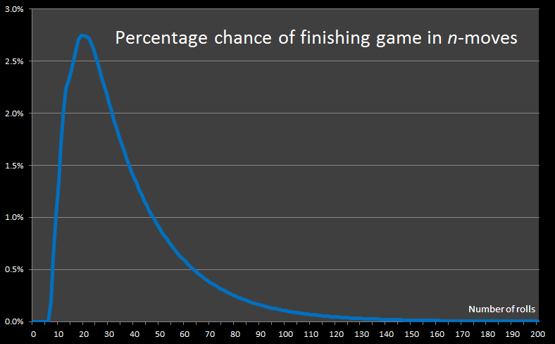
After 1 billion itterations, here is a graph of the results:
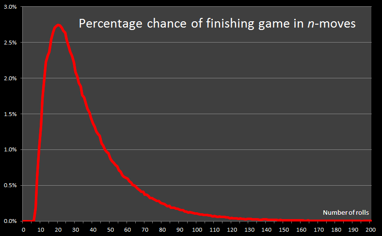
In the above graph, the x-axis shows the number of rolls, and the y-axis shows the percentage of games that were completed in that number of rolls.
The shortest possible game takes just seven rolls. There are mulitple ways this can be achieved, it happens approximately twice in every thousand games played.
One possible solution is the rolls: 4, 6, 6, 2, 6, 6, 4 This takes the user up ladder #5 which boosts the player over half the board in one go!
What kind of average are you looking for?
There are different kinds of averages.
The Modal number of rolls required to complete a game is 20 (represented by the peak on the top graph). The mode is the most frequent occurence – more games will be completed in 20 rolls than any other number of rolls.
The chart below is a plot of the cummulative probability of finishing the game by turn-n. The cummulative total, is the total of all probabilities up to and including rolln
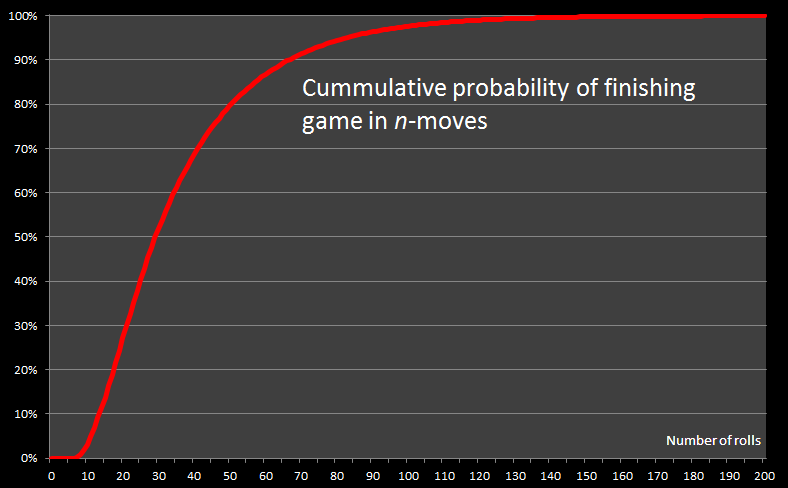
The Median number of rolls required to complete a game is 29. With a median of 29, this means that there are the same number of games that are completed in less moves than 29 as there are games that take more than 29 moves to complete.
To complete the average trifecta, we'll calculate the Mean. The (arithmetic) mean is simply the sum of all the rolls of the die divided by the number of games played. During the billion simulated games played, the die was rolled a total of 36,203,113,327 times which results gives an average of the number of die rolls per game of approx 36.2
Not all ladders are equal
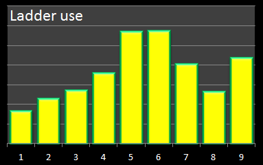
Each time a ladder (or snake) was used in the simulation, I incremented a counter for that entity to get an indication of the most 'popular' entities, and the relative frequency of their uses.
[Note - This is a count of the number of times that each ladder/snake was used, not a sum of boolean values of "Did this entity get used in this game". There is a subtle difference. If the same snake was encounterd three times in a single game, the count for this snake would be increased by 3, not just 1 ("Used or not in this game"). Think of it like a "Toll" charge for using the ladder or snake.]
Here are the histograms of their uses:
 |
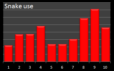 |
The least frequently used ladder, not surprisingly, is ladder#1 which can only be used if a player rolls a 1 on their initial roll. If a 1 is not rolled on the first roll, it is impossible to come back to this square. Refreshingly, looking at the count of the number of times this ladder was used in the entire simulation run results in a percentage of 16.667% – this is exactly the result we would expect since it corresponds to the 1 in 6 chance of rolling a 1 on the first roll of each game!
The next least used ladder is ladder#2. Again, not a surprise since, like ladder#1, once passed, there is no way to return to take it again. Unlike ladder#1, however, there is more than one way of getting onto this ladder over a series of early rolls, so the percentage this ladder is used is higher than ladder#1.
Limitations of an Objective approach
Objective approaches often work extremely well, but there are some limitations. Sometimes, for instance, it is simply not possible to repeat an experiment multiple times. Sometimes you only get one shot.
 |
You’re also at the mercy of your random numbers. Even assuming you have a “fair” random number generator (a topic for a whole other blog posting!) if some of the paths in your code occur with very low probability then a sufficiently larger number of iterations need to be performed to make sure these paths are given the chance to exercised proportionately. The work around for this leads us neatly to an alternative mechanism for calculating the distribution of expected game lengths. We’re going to look at subjective way to model the game of Chutes and Ladders |
Subjective Approach – Markov Chains
We’re going to use the theory of Markov Chains to compute the exact expected length of the game.
|
Games like Chutes and Ladders are ideal candidates for Markov Chain analysis because, at any time, the probability of events that will happen in the future are agnostic about what happened in the past. If a player is on grid square 18 of the board, the probability of what will happen on the next roll is independent on how the player got to square 18. It is this memorylessness that enables Markov chain analysis to work. It’s easy to see how Chutes and Ladders differs, for instance, from a single-deck game of Blackjack at a casino. In Blackjack, the probability that events will occur in the future, and thus what your optimal strategy is, is dependent on the cards that have already been played – it is for this reason that card counting works … but we’re digressing … |
 |
Stochastic Processes
At the heart of Markov Chain analysis is the concept of a Stochastic Process. This is just a fancy word to say that, from a given state, there are a series of possibilities that could happen next, defined by a probability distribution. (Implied in the definition is that all the probabilities add up to 1.0 – something will happen next).
In a game of Chutes and Ladders, a player can be on a particular square. We don't care how they got there, we just know that they roll the die again and act based on the results of the roll.
If a player is at grid square G when he rolls again, one of six things could happen (with equal probability), and based on these probabilities the player would advance to one of the next squares.
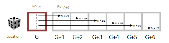
These probabilities can be represented as a sparse matrix which records the probability of moving from GridSpacei to GridSpacej by the entry in row-i and column-j. We'll call this the Transition Matrix. A vanilla snippet of this matrix can be seen below. (When there are no snakes or ladders to clutter the board, it's simply six consecutive probabilities of 1/6)
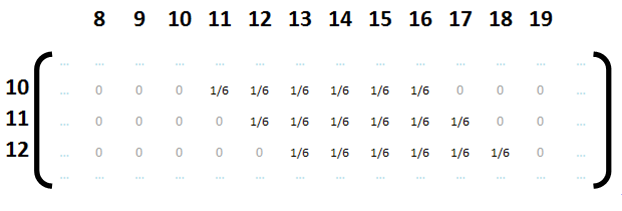
Things get a little more interesting when we add Snakes and Ladders into the mix. Now there is a chance that a roll will land a player onto the business-end of one of these special entities and they will get 'teleported' to a new location.
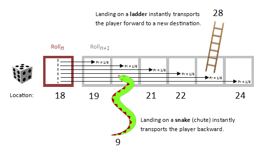
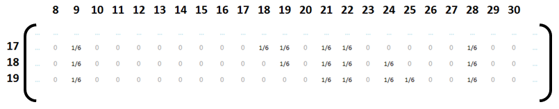
An example of the what the transition matrix would look like in this ficticious location is shown below. There are still six possible outcomes with equal probability of 1/6, but this time, rather than being consecutive, they sometimes record the locations that would be jumped to if the player would have landed on the snake or ladder. Looking at row 18 we see there is a 1/6 chance of moving to square 19, a 1/6 chance of moving back to square 9 after landing on the snake that start on square 20, a 1/6 chances of moving to squares 21, 22 and 24, and a 1/6 chance of landing on square 28 after taking the ladder from square 23.
There are just a couple of other scenarios we need to correctly address and we’ll be able to construct a full stochastic transition matrix for our game.
 |
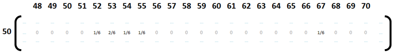
The first is the condition where it’s possible to land in a location by more than one means from a single roll. An example of this can be seen on row 50. A roll of 3 will take the player to square 53, but a roll of 6 will also land the player on square 53 (because landing on square 56 is the head of a snake which slides the player back to 53). Thus, the probability of moving from square 50 to square 53 is 2/6 and not 1/6. This is shown in the matrix snippet below. |
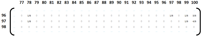
The second condition to care about is the boundary scenario when the player is close to the finish. Here, according to our house rules, as an exact roll is not needed, there are multiple ways to get to square 100. In the matrix snippet below you can see the probability of moving from square 97 to square 100 is 4/6. (And watch out for the snake on square 98 which slides you back to square 78!)
Transition Matrix
After putting in the stochastic probabilities for each square, the result is a transition matrix that is (101 x 101) and is sparse in nature. It’s (101 x 101) rather than (100 x 100) because there is a square 0 which represents the off-board starting position. (Tokens start off-board, then the first roll lands the player on the board).
|
The smarter readers amongst you will may have already have released that actually we don’t need a matrix that (101 x 101) and can, instead, represent the transition matrix as a sparse (82 x 82) grid. Why? Well the simple explanation is that it is impossible for a player to rest on the head of a snake or the bottom of a ladder. These squares don’t need to be defined as separate states since landing on them instantly transports the user to their other ends. In the (101 x 101) matrix these rows and columns are full of redundant zeros. (You can see this in row98 above). Interestingly removing these redundant rows makes a non-trivial difference to calculation speed. Matrix multiplication (which as we will see below is used for this calculation) is O(n3) so reducing the size of a square matrix from 101 to 82 doubles the speed! |
 |
The transition matrix encapsulates the probability of moving from any square to any other square.
Now, all we need to do is provide it with an input. A player starts the game off board, and nowhere else, so we create a column vector with 1.0 in the row0 (There is a 100% probability that the player will start at position zero).
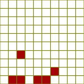
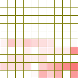
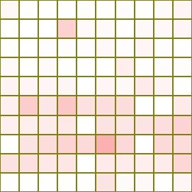
Next we multiply our column vector by the transition matrix, and the vector produced at the output is the probability distribution at the end of roll1. Each row value in the output vector is the probability that the player token will be in that square at the end of that roll. I’ll represent this graphically in the board below.
|
On the grid, non-zero probabilities are painted in red. The stronger the probability, the more intense the colour. After one iteration (multiplication), the results are pretty palpable. There are six shaded squares, each with equal probability representing the squares that would have been achieved with each distinct roll of the die. You can see that two of the rolls resulted in the use of ladders. |
|
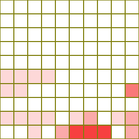
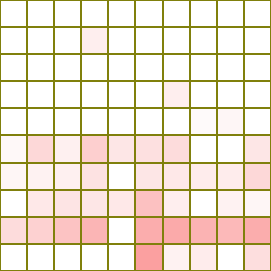
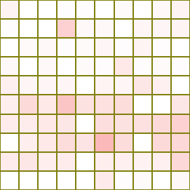
You should be able to see where we’re going with this now. We can use the output of the first roll as the input for the second roll. The output of the first roll shows the probability density of the grid. If we multiply probability density by the transition matrix again our output will be the probability density after two rolls (A superposition of all the probabilities from rolling the die again from every position on the grid). Already the probability ‘cloud’ is spreading out. The dark shading of some of the cells (especially on the lower row), highlight the superposition of probabilities and show how these spaces are more likely to be occupied after two rolls because of the multiple ways to get there. |
|
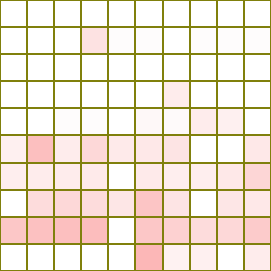
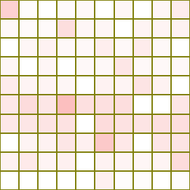
Repeating this again, we get the state after three rolls. |
|
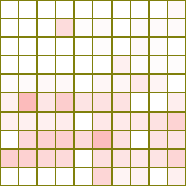
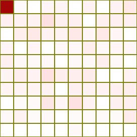
Four. |
|
Five. |
|
Six. |
|
Seven. Here we can see that (or maybe not, it's pretty faint!), for the first time, square 100 contains a non-zero value. Seven rolls is the least number of rolls required to complete the game, and it is the first time that our probability cloud reaches this square. |
|
Eight. |
|
Continuing on, here is a picture of the board after 10 rolls. You can see the colour in square 100 getting deeper, as more and more games reach completion and the probability that a game would be completed increases. |
|
Here we are after 20 rolls. The pure-white squares show the start cells of the ladders and snakes. It is impossible (zero probability) for player to be on one of these squares. The very light cells are the ones with almost no chance of the player residing in them. |

|
By 100 rolls, it's pretty much GAME OVER |
Animation
I’ve created a short animation which cycles through the probability density for rolls up to 100.
Results
To calculate the probability of completing a game after n-turns, we can examine the value in row100 of the output matrix after the initial identity input column vector has been multiplied by the (TransitionMatrix)n.
Here is a graph of the results:
Notice the curve? Yes, it’s pretty close to the curve obtained by the Monte-Carlo simulation. Actually, it's very close indeed. The only difference is that, not surprisingly, the Monte-Carlo is slightly less smooth.
The curves are so close that when I plot them both the same graph, the lines obscure each other. To differentiate them, I've made the Markov generated line a little thicker and show a zoomed in portion of the curve in the image below.
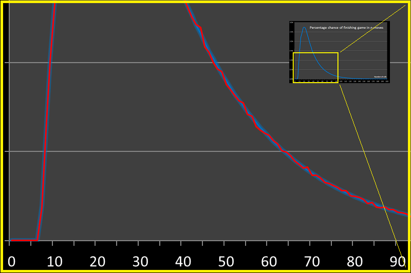
The fact that the curves are so similar (despite being generated in two very different ways) cooroborates that our code is working correctly. It also confirms that the number of simmulations we ran for the objective analysis was an appropriate number. Finally, it attests that the RNG (Random Number Generator) that shipped in Visual Basic passes at least one of the tests about generating "Good" random numbers.
Sensitivity to Changes
Now that I have a test-frame for running simulations it's easy to tweak the game and see the changes to the expected results. Generally, adding ladders to the game shortens the average number of moves, and adding addition snakes lengthens the average number of moves to complete. But that is not always the case!
 |
Initially this sounds paradoxical and counter intuitive. How can adding a snake reduce the number of steps required to complete? After all, if you don't land on the new snake, it makes no difference to the number of moves, but if you do land on it, it sends you backwards! What's going on? Well, if the snake in question happens to send you back to before the start of a really long ladder that you previously missed, it gives you another chance to take this upwards boost. Similarly, if a new short ladder is added that makes the user bypass a much longer ladder, then the small boost gained by taking the short ladder is outweighed by the chance of taking the big one. Adding too many new snakes or ladders before a significantly longer one also makes a noticable difference to the average moves. With a long clean run-up to an important entity there are multiple combinations of rolls that will land the player on that square. With many obsticles in the way, a smaller set of combinations of rolls will make it through to the start of that entity. |
You can find a complete list of all the articles here. Click here to receive email alerts on new articles.
© 2009-2013 DataGenetics