
Hilbert Curves
|
This is an article about Hilbert Curves. Hilbert Curves are named after the German mathematician David Hilbert. They were first described in 1891. A Hilbert curve is a continuous space-filing curve. They are also fractal and are self-similar; If you zoom in and look closely at a section of a higher-order curve, the pattern you see looks just the same as itself. An easy way to imagine creation of a Hilbert Curve is to envisage you have a long piece of string and want to lay this over a grid of squares on a table. Your goal is to drape the string over board so that the string passes through each square of the board only once. |
|
The string is not allowed to cross over itself. There are many patterns to achieve this effect, but Hilbert Curves have some additional interesting properties. To understand these properties, we need to take a closer look about how they are recursively defined. |

|
|
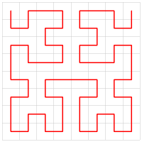
The Hilbert Curve that fits in an 8 x 8 grid is show to the left. |
Recursion
 |
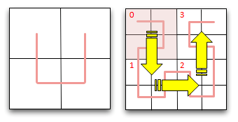
The basic element of a Hilbert curve is a U-shape. Look at the image to the left. Here we have a 2 x 2 square grid. We start with our ‘string’ in the top left corner, and drape it through the other three squares in the grid to finish in the top right corner. |
|
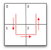
Now imagine that we double the size of the grid to make a 4 x 4 grid. We can represent this 4 x 4 grid as a nested set of 2 x 2 grids, each of size 2 x 2 (Like a set of Matryoshka dolls). We want to traverse the grid at a high level following the 0->1->2->3 coarse pattern (shown by the big yellow arrows), and then within each of these grids, with a finer self-similar traversal pattern through each of the smaller grids. |
 |
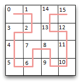 |
The result of this is shown on the left. This convoluted and snaking pattern passes through every square on the grid. |
|
If you scroll back up to look at the image of the 8 x 8 curve drawn above you will see that this follows the pattern of four 4 x 4 grids drawn in the U-shaped manner … |
 |
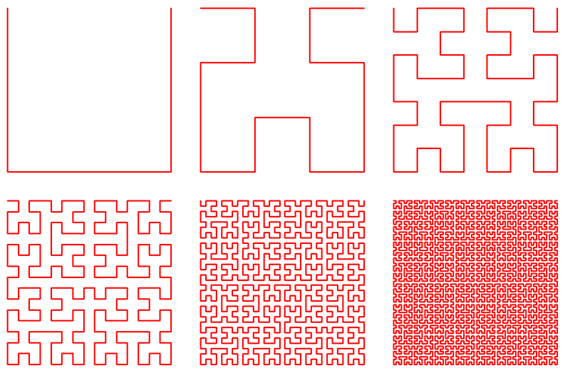
Here are some renderings of Hilbert Curves with ever increasing density:
1D into 2D
 |
Now it gets a little more interesting. Instead of using a piece of string, imagine that we are draping a measuring tape over the grid. |
Because the tape snakes and double-backs against itself around the grid it creates and interesting property: We find that if we convert the distance (d) shown on the tape-measure to a pair of (x,y) coordinates on the grid, then we find that other marks on the tape measure (close to d) have (x,y) coordinates that are very close.
We have created a useful mapping function between one-dimension and two-dimensions that does a good job of preserving locality.
|
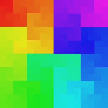
Similar values of d have similar values of (x,y) NOTE The converse can't always be true (as is inevitable when mapping from two-dimensions to one-dimension). There are bound to be cases when there are (x,y) coordinates that are geometrically close which have non-close values as measured along the tape d. However, abscent of these outliers, Hilbert Curves, in fact, do a good job at the inverse too. To the right you can see the rainbow painted, using a Hilbert Curve. Colors that are close to each other on the spectrum have similar (x,y) coordinates. (Close (x,y) coordinates don't always have similar shades of color, for the reason described above, though often they do. The discontinuities are most visible along the powers of two boundaries. Some interesting work-arounds to this limitation have been invented - more of this later.) |
 |
A closer look
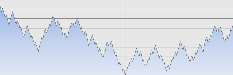
Below is a graph of the Pythagorean distance between all cells on an 16 x 16 Hilbert Curve, and a sample test point (marked with a red line). The x-axis depicts the 1D distance d as measureed along the tape. The y-axis shows the distance between the point depicted on the x-axis and the test point (marked by the red line).
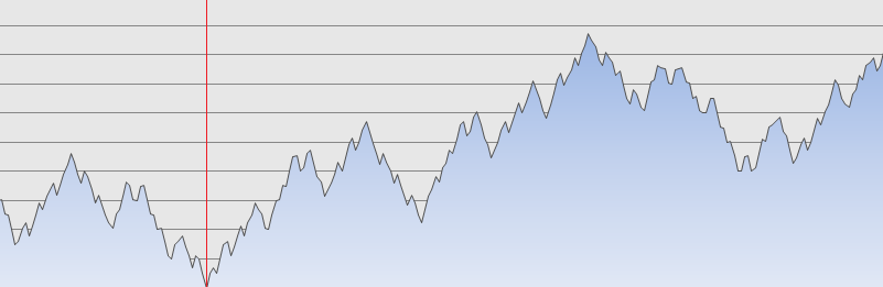
As you can see, when the value of d is close to to our test point, the distances to other points close to d is small, and the further away we move from the red line, on average, the larger the distance becomes. It's not perfect, but it's pretty good, considering how bad this might look if we'd simply zig-zagged the tape backwards and forwards like a giant Chutes and Ladders Board
In the above example, our chosen test point is 51 units in, on a scale of 0-255, where zero if the start of the tape, and 255 is the end of the tape.
Below is another example, this time with the test point at 138 units along the curve.
As before, the further away one gets from the test point, the larger the distance between the (x,y) coordinate pairs becomes. And, as before, values of d close to the test point map to coordinates that are close-by the (x,y) coordinates of the test point.
Here is a heat map showing the distance between all pairs of values of d. The brighter the color, the larger the distance. The top left of the grid represents the distance between d=0, d=0. Each pixel move to the right n represents d=n and each pixel move down m represents d=m, and the color of each pixel represents the Pythagorean distance between the two points d=n, d=m on the 2D plane.
(The graphs above are equivalent to horizontal slices through this grid with the shade of the color representing the graph height).
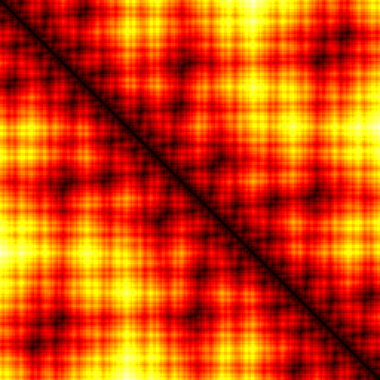
Note the dark band all the way down the leading diagonal. This shows that, for all values of d, the values that are numerically close to d are positioned with (x,y) coordiantes in close proximity.
Higher Dimensions
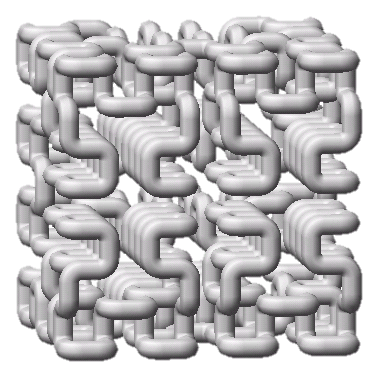 |
The characteristics of Hilbert Curves can be extended to more than two dimensions. A 1D line can be wrapped up in as many dimensions as you can imagine. A rendering of a curve in 3D can is shown on the left. In this shape, points on the line numerically close to one another are also close in 3D space. It's easy to see how this can be extended into higher dimensions.
|
Practical Uses
|
Hilbert Curves don't just look cool, they are very useful constructs. Hilbert functions can help build indexes for spatial databases; when searching for a record in close geographic location they can help determine the priority for exploring. Outside of database work, they are sometimes used in image process. When converting an image to gray scale through the dithering of black and white pixels, carry-over values from thresholding can be carried forward and, by the use of a Hilbert Curve, the excess can be distributed in a pattern less obvious to the eye. At higher dimensions they can be used to implement task scheduling in parallel processing computing applications. Converting multiimensional task allocation into a one dimensional space and assigning related tasks to locations with higher levels of proximity. |
 |
Ongoing Research
Recall I mentioned ealier that, whilst OK, the inverse look-up features of Hilbert Curves are not ideal? (Places with similar d values also have similar (x,y) values, but the converse is not always true?)
This feature would be incredibly useful, for instance, in allowing efficient accessing of data. Let's imagine you have some data stored in digital cold storage (a location with very high access times), and wish to index and access this in an efficient manner for searching geographically. As we know, converting the (x,y) coordinate into a d value might not guarantee that similar values of d are located in close proximity. Most of the time, yes, but some of the time, no.
To counteract this, rather tham simply indexing the data on a single Hilbert Curve, the data is translated onto a set of Hilbert Curves (typically a mix of rotations and horizontal/vertical translations of the same curve). In this way, by combining the results, any unfortunate edges from step-changes around the 2n boundaries are smoothed out.
XKCD
Finally, no article on Hilbert Curves can be written without referencing Randall's Map of the Internet

You can find a complete list of all the articles here. Click here to receive email alerts on new articles.

© 2009-2013 DataGenetics Privacy Policy