
Pixel Scalers
Computer images are made out of pixels (short for picture elements). A typical image displayed on a web page, for instance, is made out of thousands of individually shaded elements (usually, but not always, approximately square in shape).
In the early days of computers, resolutions of screens were quite low and individual pixels were clearly distinguishable. Today, with display technology such as the Retina Display™, the density of the pixels is so high that the human eye is unable to distinguish the individual pixels when a device is operated at regular viewing distances.
 |
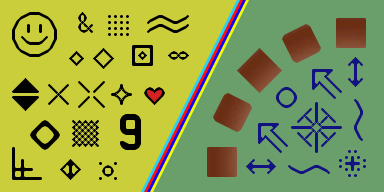
Similarly, color-depth (the number of distinct colors that each pixel can be shaded) has correspondingly increased with technology. Typically these increases have gone up in natural powers of two reflecting the binary nature of how computers store information. Early displays were described as mono-chrome, implying just one color, but technically these displays were two color devices; each pixel could be on, or off: Black or White, Green or Black, … depending on the technology used. The image on left is a low resolution mono-chrome image. |
|
Technology moved through four color display modes, then sixteen, and onto 256 color displays. Things stayed on 256 for quite a while. Interestingly for 256 displays, these initially used a palette system and, whilst there was only a maximum of 256 distinct colors allowed on the screen at any one time, each of these colors was selectable from 16,777,216 possible colors. (This number represents 256 possible shades of Red, mixed with 256 possible shades of Green, mixed with 256 possible shades of Blue). |
 |
 |
These days, most common displays allow any pixel to be any one of these 16.8 million colors, without the use of a palette, by storing the 256 values of RGB for each pixel. |
Raster and Vector
|
There are two fundamental mechanisms for how graphics can be stored for rendering on computers. These are Raster and Vector. Each has benefits and downsides. |
|
Raster images (also commonly called referred to as Bitmap images) are stored as a matrix of the individual pixels that make up the image. You always know how they will appear, and computers are optimized to display them very efficiently. Raster images, however, have some down sides: They are created at a particular size (resolution), and if you need to scale them up or down, you have to decide how to map the pixels in the source image to the different size destination image. This scaling is what I’m going to talk about in this article. A similar issue occurs if you have to rotate the image. I wrote about this issue in another fun article a few months ago. |
 |
|
Vector representation encodes a graphic, not as a collection of pixels, but instead as collection of elemental shapes. e.g. There is a line between these two coordinates, and there is a circle centered here with this radius. At render time, these instructions are interpreted and the image drawn. Rendering is much slower, but has the advantage that it is resolution independent. Vector rendering is agnostic of the resolution of the display used; the higher the resolution of your output display, the crisper the image seen. They can also scale by any factor without causing aliasing or pixilation issues (no ‘jaggies’ on un-horizontal or un-vertical lines). They can also be rotated by any arbitrary angle without issue. |
 |
(There are other technologies that can be used to store then re-render images, such a Fractal Compression, and Fourier Compression. Similar to the Vector systems, these technologies are resolution independent. Both store the image as a resolution agnostic collection of fundamental components (fractals or sinusoidal waves), which can then be used to regenerate the desired image at the required resolution. By their nature, both of these systems are lossy compression/rendering technologies).
For the rest of this article, I'm going to focus on scaling of raster images.
Arbitrary scaling of bitamps
As stated above, bitmaps are designed to rendered at one defined resolution. If a bitmap image needs to be scaled (stretched or reduced), this causes issues as the pixel blocks no longer align with the grid used to display them.
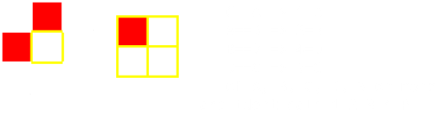
The image on the left shows a random collection of colored pixels (with thin red lines representing the boundaries of the pixels). The image on the right shows a possible situation where the image is expanded slightly.
 |
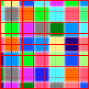 |
One simple solution (called the nearest neighbor interpolation algorithm) is to color the destination square with the color of the nearest stretched source image pixel. (Each pixel in the destination is shaded with the color of the nearest centroid of the source image after it has been projected/stretched to its new position). This algorithm is very quick to implement, and has an interesting property that the new image only contains colors that were present in the original image.
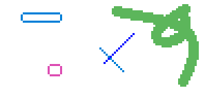
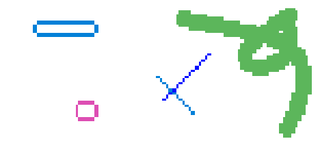
Here is an example of it being applied to scale up the collection of shapes on the left by 158% to make those on the right:
 |
 |
As well as creating obvious 'lumps' in lines and curves, it also potentially messes up the overall brightness of the image and wastes a lot of information that is stored in the picture (data from not all the source pixels is used if the image is shrunk, and if it is stretched, some data is used disproportionately more than others).
 |
The next level of sophistication is called Bilinear filtering. If you look closely at the colored patchwork sample destination image above you can see that each new destination pixel is composed from (at most) four different source pixels in various ratios. Bilinear filtering proportionally mixes the colors of these source pixels so that the destination pixel is the average of the four source images weighted by the area contribution of each source pixel. This certainly gives a smoother output than the nearest neighbor algorithm, and information from all the source pixels is used to create the destination image (preserving the overall brightness of the image), but this has the side effect that new colors are formed in the destination (for instance, a mixing of an adjacent black and white pixel in a source image would result in some shade of gray in the destination, depending on the mix of the two colors). Bilinear scaling works reasonably well when the scaling factor is not too severe (scaling ranges between 50% of original up to 200% of the original). |
An even more sophisticated system of scaling is called Bicubic filtering. Whilst in Bilinear filtering where just the four corners are used to interpolate the color of the new pixel, in Bicubic filtering, values of pixels further afield are used to determine the appropriate color.
Bilinear scaling uses (2 x 2) pixels from the source image. The "bi-" part of the name represents that the process is applied to both the x-axis and y-axis, and the "-linear" shows that the interpolation occurs be using a straight line approximation.
Bicubic scaling uses (4 x 4) pixels in the source image to determine the color of the destination pixel. By using all sixteen pixels (the four corners and pixels further afield), a more accurate representation of the shape of the curve of the colors can be determined. Again, this is applied to both the x-axis and y-axis "bi-", and the "-cubic" part tells us that a third order polynomial is fitted through the points.
He is an visualization of these two techniques (in just one axis), and shows how the different techniques give different values.
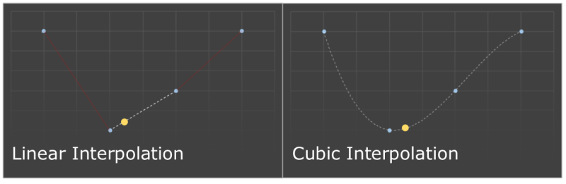
In the graph on the left, a straight line is drawn between two points (the colors of two source pixels), then the desired point (represented by the yellow dot), is read as the pro-rata weighted average using this line.
On the graph on the right, a cubic curve is fitted through four points (the two corner pixels, and the two further away). This gives a better indication of the trend of how the colors are changing. You can see this gives a slightly different result when the test point is selected.
Examples
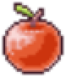
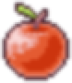
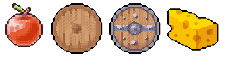
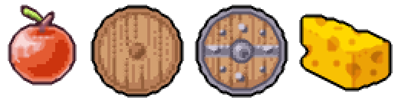
Below is an example of the application of each of these three techniques (Nearest Neighbor, Bilinear Interpolation, Bicubic Interpolation) to the image of an apple (shown on the right). I've scaled each image by 162% To enable the technique to be understood, I've also shown each of the results blown-up so you can see the individual pixels in more detail. |
 |
 Nearest Neighbor Nearest Neighbor |
 Bilinear Interpolation Bilinear Interpolation |
 Bicubic Interpolation Bicubic Interpolation |
 |
 |
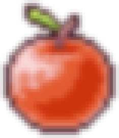 |
It's clear that, whilst the nearest neighbor algorithm does not create any new colors, the results are not very elegant. Some pixels are scaled more than once. The bilinear scaling produces much smoother results, but the image is blurred with softer edges. Individual pixels are still clearly distinguishable, and there are some obvious sharp transitions between some connected pixels. The bicubic interpolation is very smooth with nice soft gradients between pixels and is certainly the most pleasing to the eye. Here are the same results, this time with a white background, which highlights the soft edges. |
 |
 Nearest Neighbor Nearest Neighbor |
 Bilinear Interpolation Bilinear Interpolation |
 Bicubic Interpolation Bicubic Interpolation |
 |
 |
 |
Fixed Ratio Scaling
 |
There is a special case of scaling, and this occurs when the required output is an exact multiple of the source image (for instance to 2x or 3x or 4x …) This happens quite often when converting/emulating old video games to run on new consoles and computers. Older games were designed to run on computers and devices with lower resolution displays, and if displayed at 1:1 pixel ratio they would be too small to play. To solve this problem, the graphics can be easily scaled by a fixed multiple ratio. Interestingly, some quite sophisticated algorithms have been developed to handle this task (and to avoid, as much as possible, the creation of ‘jagged’ edges in the destination image). |
|
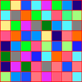
Let’s take a look at a selection of some of these algorithms applied to the sample bitmap on the right. |
 |
Nearest Neighbor
The simplest mechanism is to apply the nearest neigbor algorithm. Each pixel is simply duplicated the number of times of the scale factor. This technique is elegant in its simplicity, but produces a blocky output.

EPX
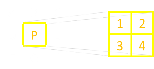
EPX is a technique named after its inventor, Eric Johnson (Eric's Pixel Expander). It was created at LucasArts in the early 1990's for converting games originally developed on the PC at a resolution of 320 x 200 to early color Macintosh devices.

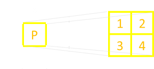
It starts out the same basic way of expanding each pixel P into four destination pixels of the same size: 1, 2, 3, 4
|
The four destination pixels are initially colored with the same color as the source pixel, then each pair of pixels up/below and left/right are compared in corners. |
 |
If the two pixels adjacent to each corner are the same color then this color overrides the color of the corresponding destination quadrant (UNLESS three of more of the pixels A, B, C, D are the same color, then the pixel remains the same as it started as color of P).
 |
The shading of the respective destination quadrant based on edges of same color helps fillet and fill in in the gaps of diagonal lines close to 45°, removing their blockyness.
 |
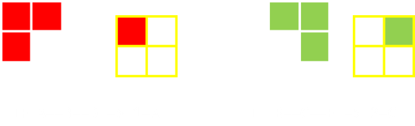
This algorithm also has the advantage that it generates no new colors: Every pixel in the destination is a representation of a colored pixel in the source image. On the left I've shown the improvement in aesthetics over the basic nearest neighbor. The left half of the image (white background) is the simple nearest neigbor solution of the left half of the apple image. Reflected on the right side is the EPX scaled version of the same image. There are enhancements to this system to cover scaling by a factor of 3x. Whilst the principle is the same, the algorithm is slightly different. |
Eagle Algorithm
A similar algorithm to EPX is called Eagle. Here is a sample output.
As before, the only colors in the destination are also present in the source. However results, typically, aren't a smooth as the EPX algorithm.
|
For Eagle, as before, the four destination pixels are all set to the same color as the center pixel in the source image. |
 |
Then, all three pixels in each surrounding corner are checked. If all of these are the same color, then the appropriate quadrant in the destination is colored the same.
 |
The Eagle algorithm has an undesirable feature (bug?) that a single pixel surrounded by eight pixels of the same color will disappear! There are different enhanced versions of Eagle available that correct this issue.
One of these Eagle enhanced/inspired family of algorithms is called SaI. Here is an implementation of a Super SaI version of the algorithm:
The SaI algorithms were developed by Derek Liauw Kie Fa a.k.a Kreed. You can see that these algorithms also blend the output pixels and so colors not present in the original are rendered. The Super SaI implementation looks at pixels further afield than just the eight nearest neighbors to help it determine if there are lines/commonalities at different gradients that need to be taken into account.
HQx family
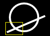
The HQx family of algorithms were developed by Maxim Stepin. There are various versions (hq2x, hq3x, and hq4x) for scale factors of 2:1, 3:1, and 4:1 respectively. Each algorithm works by comparing the color value of each pixel to those of its eight immediate neighbours, marking the neighbours as close or distant, and then uses a pre-generated lookup table to find the proper proportion of input pixels' values for each of the 4, 9 or 16 corresponding output pixels. The hq3x family will perfectly smooth any diagonal line whose slope is ±½, ±1, or ±2 and which is not anti-aliased in the input; one with any other slope will alternate between two slopes in the output. It will smooth very tight curves.
Here it is on our sample image:

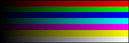
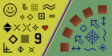
It's a pretty elegant algorithm. Here is output generated by the hq3x version on a different test card:
 |
 |
I think you will agree, these results look awesome!
xBR Family
The xBR family of algorithms work in a similar way to the HQx algorithms (using lookup tables for pattern recognition). However, they go further than HQx by using a 2-stage set of interpolation rules. These better handle more complex patterns such as anti-aliased lines and curves. Background textures keep the sharp characteristics of the original image rather than becoming blurry like with HQx.
There are two implementations of xBR. One uses blending (the top image below), and the other no blending. The blended implementation creates smooth anti-alised outputs, but creates additional colors. The no blend version only uses colors present in the source image.


This algorithm works by detecting edges and interpolating pixels along those edges. It determines edges as pixel regions in the image where pixels are very distinct/different along some direction (high color frequency) and very similar perpendicular to that direction (low color frequency).
There is even an optimized version of xBR, called xBRZ (developed by Zenju), that attempts to preserve small pixel details that are common in faces.
Comparison of 4x algorithms
Below are comparisons of nearest neighbor (left), HQ4x (middle) and 4xBR.
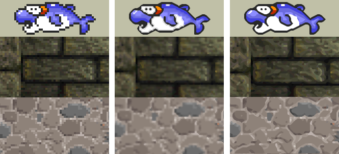
Very cool indeed. For more details, check out this awesome paper.
You can find a complete list of all the articles here. Click here to receive email alerts on new articles.
© 2009-2013 DataGenetics Privacy Policy