
The Secretary Puzzle
|
This problem is given many names. Sometimes it is called the Secretary Puzzle, sometimes it is called the Wife Puzzle, sometimes the Marriage Problem, sometimes the Googol puzzle, sometimes the Interview Puzzle … No matter the name, the concept is the same. It’s an easy problem to state, a medium difficulty problem to analyze, and a thoroughly fascinating problem to investigate as an example of statistics, probability and decision making. He're we go … |
 |
Statement of Problem
 |
You are interviewing to select yourself a new secretary (or wife, or husband …), and there are n candidates applying for the position. The potential suitors are all waiting in the next room. You interview them individually, one-by-one, in a random order. After each interview, you must make a binary decision: HIRE or PASS. If you select HIRE, the interview process immediately stops as you have only one position to fill. If you PASS on a candidate, they are dismissed, they leave the interview room, and you do not get a second chance with this applicant (They are passed by for good). |
GOAL: The aim of the exercise is to try to select the very best candidate from the applicant group.
You have no idea of the distribution of talent in the pool, but you do know the total number of candidates. What is the optimal strategy to maximize your chances of selecting the top candidate? What is the probability of success with this strategy? What happens to this strategy as n changes?
Analysis
In order to simplify analysis, we’ll convert the talents of each candidate into an ordinal number (there are no ties). Each potential secretary being represented by a distinct number from 1 – n. The higher the number, the more desirable the candidate.
e.g. Here are 16 candidates in random order: 5 13 1 12 16 3 4 6 15 7 9 10 11 14 2 8
 |
If you selected totally at random, the chance of this subject being the very best candidate is 1 / n. This is also the chance if you selected the first candidate you see (There is a 1 in n chance that the first person you see is the best contender). |
|
After thinking about this for a little while, we can see that a better strategy is to meet a few candidates, take notes of their talents, remember the highest, then continue through the rest of the candidates, and select the next one we see whose skills exceed the highest we encountered in the sample set. |
 |
The idea of taking a sample first is a good one: By looking at a sample of the candidates first, we can get some idea of the range/distribution of their skills. But … What sample size should we take?
Too small a sample and we don't get very much information about the set. Too large a sample, and though we get plenty of information, we've burned too many of the potential candidates to get this knowledge, leaving very few to choose from. In words of baby-bear, what sample size is “Just right” ?
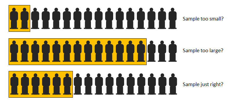
There's also a more subtle issue if we get the sample size incorrect (because of the fact that we can only select one candidate).
|
If our sample size is too small, then the number of candidates not in the sample is large. Because our strategy is to select the first candidate whose skill exceeds the highest we saw in the sample, there is a good chance this may occur before the ideal candidate is seen. |
 |
 |
Similarly, there is an issue if the sample size is too large. With too large a sample there is a good chance that this sample will include the best candidate! |
(If this occurs, then we'll end up with the last candidate seen. What else can we do?)
 |
The optimal solution will be to suggest an appropriate sized sample to examine that is big enough to allow enable us to estimate what is a “good” candidate, but not so large as to have a high chance of including it (and also not so low that we end up taking the first “potentially good” candidate we see and stop before reaching the best). Other canonical Forms Whilst we'll use the ‘secretary’ version of the puzzle today, you can see how determining an optimal sample/stopping point is analogous to other versions of the puzzle (selecting a wife, husband, job applicant, best pizza …) |
In the Googol Puzzle variant, your friend selects n pieces of paper, and on each one writes a different number. These are then placed in a basket and mixed up. Your task is to draw them, one-by-one, from the basket and decide when to stop, with the aim of stopping holding the piece of paper that contains the highest number! |
 |
Walkthrough
Before delving deeper into the math, it's worth hand-walking through this problem for small sizes of n to fully appreciate the push and pull of the various constraints of the puzzle.
n = 1
This is a trivial case. We select the one and only applicant. By definition, we'll get the best candidate that applies!
n = 2
This case is also trivial. It's a coin-flip. There is a 50:50 chance of selecting the best candidate. It does not matter what you do. There is no optimal strategy. Either the first candidate you see is the best, or they are not.
If we elect to not sample (sample size = 0) then we select the first candidate we see. 50% of the time we'll be correct, and 50% of the time we will not be.
If we elect to sample (sample size = 1) then we look at the first candidate. 50% of the time the second person we see will be higher that the first, and 50% they will not be.
Therefore, it does not matter if we sample or not with n = 2
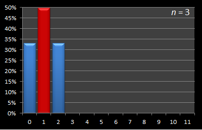
n = 3
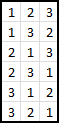 |
This is the first non-trivial example, and one where we can start to apply strategy. With three candidates, there are six possible combinations that our candidates could appear in (3 factorial for my mathematical readers). First let's write down all possible combinations. Here they are shown on the left. We have three possible strategies. There are three possible sizes of sample sizes we can select from. These are: 0, 1, 2 |
|
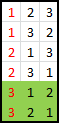
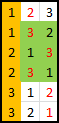
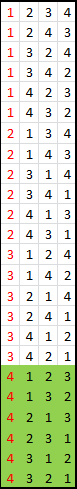
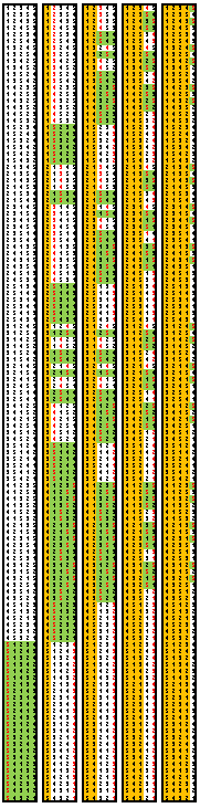
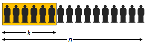
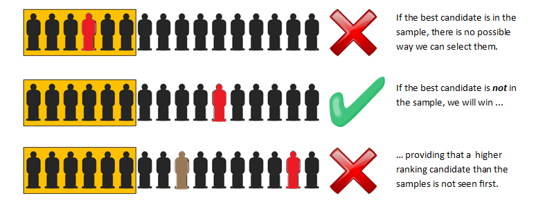
Let's look at the three possible sample sizes, and for each, determine how many of these would result in us selecting the best candidate. In the diagrams below, the ORANGE BOX represents the sampled candidates, the RED number represents the candidate selected by the algorithm. The GREEN BOX shows the rows for which this solution results in the best candidate being selected. |
|
n = 3, Sample Size = 0 Our algorithm tells us to select the fist encountered candidate higher than any found in the sample, since there is no sample this has to be the first candidate encountered. 2 times out of 6 is this the best candidate. With a sample size of zero, we select the best candidate 2 / 6 times. |
 |
|
n = 3, Sample Size = 1 Here we sample the first candidate, then select the next candidate who appears that exceeds this value. As you can see, if we were unlucky enough to encounter the best first, we can never recover, but otherwise, we only fail if the other candidates are in numeric order. With a sample size of one, we select the best candidate 3 / 6 times. |
 |
|
n = 3, Sample Size = 2 Here we sample the first two. As you can see, this only results in picking the best candidate only when the last candidate is the best candidate. With a sample size of two, we select the best candidate 2 / 6 times. |
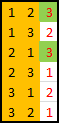 |
Result! We have an optimal strategy. Using a sample size of one we can make our chances of success 3/6 (a 50:50 chance). This is higher than any of the other sample size strategies. Thus, if are interviewing and there are just three candidates we should set our sample size to one. Let's keep going …
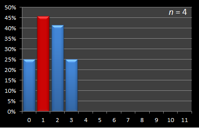
n = 4
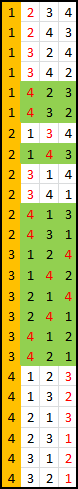
With four potential candidates there are 24 possible interview order combinations, and four possible sample size strategies (0, 1, 2, 3). Let's repeat the exercise above with our larger universe. Here they are displayed below:
Sample Size = 0 |
Sample Size = 1 |
Sample Size = 2 |
Sample Size = 3 |
 |
 |
 |
 |
Success = 6 / 24 |
Success = 11 / 24 |
Success = 10 / 24 |
Success = 6 / 24 |
As you can see from the above analysis, again there is an optimal strategy. With a sample size of one, our expected success rate is 11 / 24 situations. This is higher than any other sample size (and also an impressive 45.8% chance of selecting the best candidate).
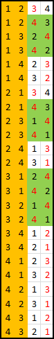
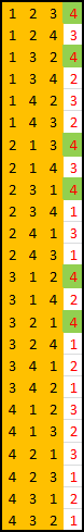
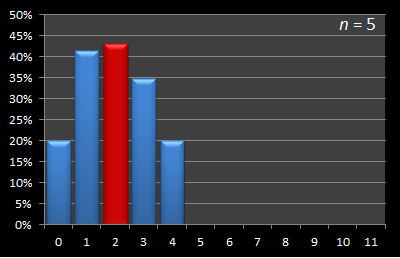
n = 5
With five candidates, the number of permutations increases to 120.
 |
I've shrunk the tables down to fit them on screen, and they are shown on the left. Here are the results in tabular format:
As always, with the sample size zero, the odds of selecting the best candidate are the same as randomly selecting (as it is when the sample size is n - 1). These odds represent the chance that the first or last seen candidate (respectively) is the best candidate. However, the optimal strategy to maximize the chances of selecting the best candidate has increased to a sample size of 2. There are two more chances of selecting the best candidate (52/120) with this sample size cf. a sample size of 1 (50/120). When interviewing five candidates, the optimal strategy is to sample the first two candidates before making decision. |
n = 6
With six potential candidates, the number of combinations increased to 720. Here are the results:
| Sample Size | Success Rate |
|---|---|
| 0 | 120/720 |
| 1 | 274/720 |
| 2 | 308/720 |
| 3 | 282/720 |
| 4 | 216/720 |
| 5 | 120/720 |
Again, the optimal strategy is to take a sample of size two.
It's a fun little programming exercise to write code to reproduce these results by enumerating out all the combinations. Interestingly, when I did it I found many parallels with the code written to solved the Eight Queens Problem. (In the Queen's puzzle you want to make sure there is only one Queen on each rank and file before testing the diagnols, and rather than brute-forcing all combinations, you simply want your solutions to start with this assumption. I make reference to this in the earlier article as the “Eight Rooks” puzzle).
n = 7, 8, 9, 10, 11, 12
Continuing on with ever increasing number of candidates …
| Sample | n = 7 | n = 8 | n = 9 | n = 10 | n = 11 | n = 12 |
|---|---|---|---|---|---|---|
| 0 | 720/5,040 | 5,040/40,320 | 40,320/362,880 | 362,880/3,628,800 | 3,628,800/39,916,800 | 39,916,800/479,001,600 |
| 1 | 1,764/5,040 | 13,068/40,320 | 109,584/362,880 | 1,026,576/3,628,800 | 10,628,640/39,916,800 | 120,543,840/479,001,600 |
| 2 | 2,088/5,040 | 16,056/40,320 | 138,528/362,880 | 1,327,392/3,628,800 | 13,999,680/39,916,800 | 161,254,080/479,001,600 |
| 3 | 2,052/5,040 | 16,524/40,320 | 147,312/362,880 | 1,446,768/3,628,800 | 15,556,320/39,916,800 | 182,005,920/479,001,600 |
| 4 | 1,776/5,040 | 15,312/40,320 | 142,656/362,880 | 1,445,184/3,628,800 | 15,903,360/39,916,800 | 189,452,160/479,001,600 |
| 5 | 1,320/5,040 | 12,840/40,320 | 127,920/362,880 | 1,352,880/3,628,800 | 15,343,200/39,916,800 | 186,919,200/479,001,600 |
| 6 | 720/5,040 | 9,360/40,320 | 105,120/362,880 | 1,188,000/3,628,800 | 14,057,280/39,916,800 | 176,402,880/479,001,600 |
| 7 | 5,040/40,320 | 75,600/362,880 | 962,640/3,628,800 | 12,166,560/39,916,800 | 159,233,760/479,001,600 | |
| 8 | 40,320/362,880 | 685,440/3,628,800 | 9,757,440/39,916,800 | 136,362,240/479,001,600 | ||
| 9 | 362,880/3,628,800 | 6,894,720/39,916,800 | 108,501,120/479,001,600 | |||
| 10 | 3,628,800/39,916,800 | 76,204,800/479,001,600 | ||||
| 11 | 39,916,800/479,001,600 |
As you can see, the optimal strategy for sample size is increasing with increasing n.
By the time the number of candidates has increased to eight, the optimal strategy has increased the sample size to three. It increases to four at n = 11.
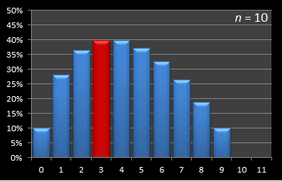
Graphs
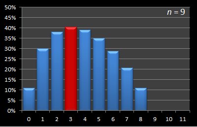
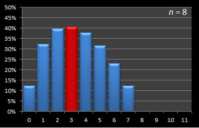
Here is this data presented in graphical format. Below are a series of graphs with values of n from 12 to 3. The x-axis shows the sample size, and for each of these samples, the percentage chance of being able to select the best candidate with this strategy is displayed on the y-axis. The optimal sample size for each experiment is shown in red.
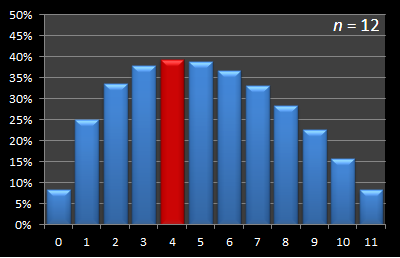 | 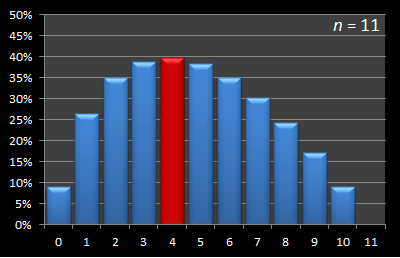 |
 |  |
 | 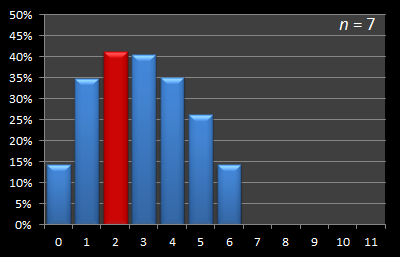 |
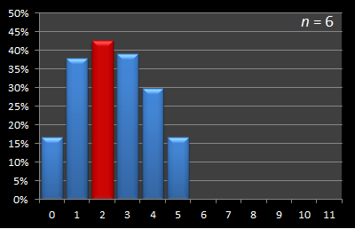 |  |
 |  |
Switching to percentages
The fractions make the values hard to appreciate (and also their relative sizes hard to comprehend), so we'll switch to decimals and percentages. Below is a table showing the the results of the first few values of n.
For each number of candidates, I've calculated the optimal sample size. From this point on, we'll represent the size of the sample with the variable k. The optimal k is shown for each row. You can see that k increases as n increases.
The next colums shows the ratio of k / n as a percentage – what percentage of the total candidates does the optimal sample represent?
Finally, the last column in the table shows the percentage chance that employing the optimal sample size strategy will enable us to select the best candidate.
|
 |
I don't know about you, but I'm pretty surprised with how high the success percentage chance is!
Over 38% success rate of selecting the very best candidate by employing this strategy with twenty applicants – nice!
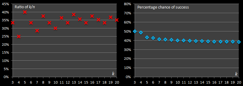
Looking at the graph, the success percentage appears to be asymptoting close to a 37% chance rate, interestingly as does the ratio of k / n. (The graph on the left is initially very 'up/down', as it is created by the ratio of k/n, and there is no concept of fractional candidates. When n is small, it has to 'snap' to the nearest round number).
To see how if this pattern continues we need to formulate a more general mathematical representation of this problem.
General Solution
Working through all the combinatronics and permutations of the ways that n candidates can be arranged is fun, but not very scalable. We need a new strategy for calculating the optimal solution. Let's go back to basics. Recall from before what conditions are necessary for success:
If our best candidate is in the sample window, it's game over. There is nothing we can do to recover from this situation.
If this does not occur, our chance of successfully selecting the best candidate is based on the chance that we encounter this before one higher than the sample is encountered
|
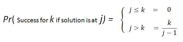
Let's look at a general case. We'll introduce a test subject in position j. We need to work out the probability of success, if our candidate was in this position, for all possible values of k. Firstly, we'll simply examine what it would take to make j a potentially ‘valid’ solution irrespective if it is the best candidate or not. |
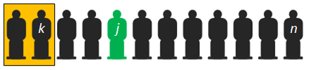 |
If j ≤ k there is no chance. If j > k, then a sample strategy of k being successful is possible if, and only if, one of the first k candidates (the ones that are automatically rejected) is the best amongst the first j - 1
 |
To be even potentially successful, we need to make sure that out of the first j-1 candidates that one of the first k candidates is higher. |
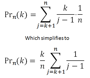
Next we know that there is an 1 / n chance that our test subject j is the the best candidate. Therefore to calculate the final probablity we need to sum the conditional probabilities for each posible position (multiplied by the 1 / n chance for each location).
|
The formula is shown on the right, and with simplification we can extract the k / n term (the ratio of the sample size to the number of candidates). As n gets larger, the summation more closely approximates a Riemann integral. There's a cute animated gif on Wikipedia showing this concept. View it here. We can approximate the integral (area under the curve; the sumation of the individual probabilities), as collection of thin ‘slices’ of width 1 / n (See below) 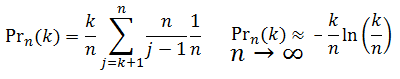
|
 |
.gif)
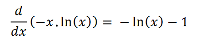
Finally, a little calculus. We want to find the maximum value for Prn(k) If we substitute x = k/n and differentiate (using the helpful product rule) we get the following:
Setting this to zero allows us to determine the value for x which is the maximum. (After confirming, of course, that the d2/dx2 is negative!) |
 |
Results
Setting the first differential to zero results in a value for x of 1 / e.
Below is a graph for for a reasonably large value of n (400) and you can see the shape.
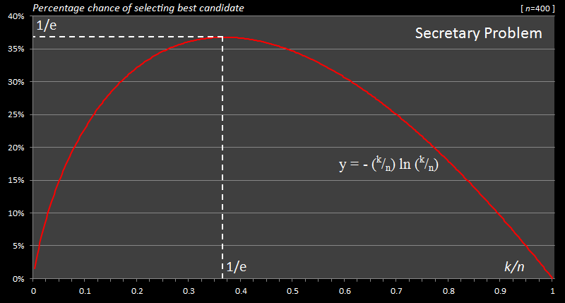
As you can see from the graph, and our calculus, the optimal sample size strategy is a 1 / e value for the k / n ratio, which corresponds to approximately 36.79% Interestingly, the chance of success when adopting this strategy is also 36.79%!
Summary
 |
When interviewing blind for a position, skip the first 36.79% candidates you meet, then select the first candidate you see whose talents exceed the highest you've seen to-date. There is a 36.79% chance that you will end up with the best candidate in the set! |
You can find a complete list of all the articles here. Click here to receive email alerts on new articles.
© 2009-2013 DataGenetics