
Battleship
I’m going to continue my analysis of classic card and board games by looking at the game of Battleship. (See early postings for analysis of Chutes & Ladders, Candyland and Risk).
|
Battleship is a classic two person game, originally played with pen and paper. On a grid (typically 10 x 10), players ’hide’ ships of mixed length; horizontally or vertically (not diagonally) without any overlaps. The exact types and number of ships varies by rule, but for this posting, I’m using ships of lengths: 5, 4, 3, 3, 2 (which results in 17 possible targets out of the total of 100 squares). |
|
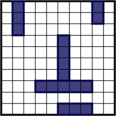
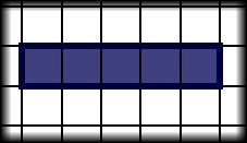
A couple of example layouts are shown below:
 |  |
Not overlapping, but touching
|
Note: even though ships cannot overlap, there is nothing in the rules to say they cannot touch. (In fact, some players consider this a strategy to confuse an opponent by obfuscating the true layout of ships. If there are five ‘hits’ in a row, a naive player might consider this to be the successful destruction of an aircraft carrier of length 5, but actually it could be the sinking of a battleship of length 4, and part of a cruiser of length 3) |
|
Simple Game Rules
|
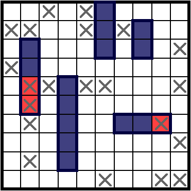
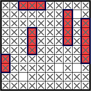
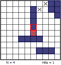
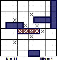
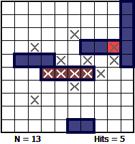
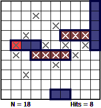
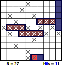
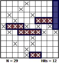
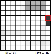
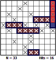
We’ll start with a description of the simplified method of play: After each player has hidden his fleet, players alternate taking shots at each other by specifying the coordinates of the target location. After each shot, the opponent responds with either a call HIT! or MISS! indicating whether the target coordinates have hit part of a boat, or open water. An example of a game in progress is show on the left. In these diagrams, misses are depicted by grey crosses and hits by red squares with grey crosses. The first player to sink his opponent’s fleet (hitting every location covered with part of a boat) wins the game. |
Random Play
The first possible strategy for building a computer opponent is to make shots totally at random.
|
As expected, the results of firing random volleys produces very poor results. Games take a long time to complete, as the majority of squares have to be hit in order to ensure that all the ships are sunk. |
Mathematically, the chances of playing a perfect game with random firing are easy to calculate and are:
355,687,428,096,000 / 2,365,369,369,446,553,061,560,941,772,800,000
(This equates to, on average, once in every 6,650,134,872,937,201,800 games!)
I ran 100 million simulations of random games, and the smallest number of moves I encountered was 44 shots.
Below is the graph showing the distribution of the number of random shots required to finish each of the 100 million simulations. The x-axis shows the number of shots, and and the y-axis shows the number of games that were completed in that number of shots.
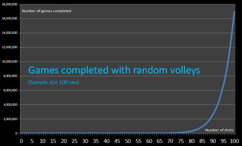
(It should be no surprise that number of games that required all 100 shots to be fired is 17 million. After all, there is a 17/100 chance that the last square visited will contain a ship).
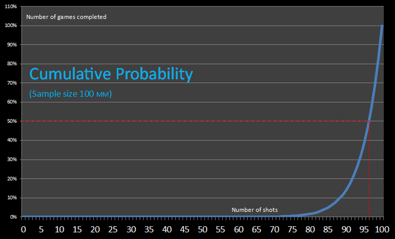
Below is a graph of the cumulative probability of completing the game with n-random volleys. 96 shots are required to complete approx 50% of the games, and 99% of the games will take more than 78 shots.
A better strategy
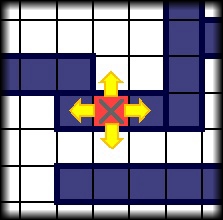
It's fairly easy to greatly improve results. Initially, shots can be fired at random, but once part of a ship has been hit, it's possible to search up, down, left and right looking for more of the same ship.
|
A simple implementation of this refined strategy is to create a stack of potential targets. Initially, the computer is in Hunt mode, firing at random. Once a ship has been 'winged' then the computer switches to Target mode. After a hit, the four surrounding grid squares are added to a stack of 'potential' targets (or less than four if the cell was on an edge/corner). Cells are only added if they have not already been visited (there is no point in re-visiting a cell if we already know that it is a Hit or Miss). Once in Target mode the computer pops off the next potential target off the stack, fires a salvo at this location, acts on this (either adding more potential targets to the stack, or popping the next target location off the stack), until either all ships have been sunk, or there are no more potential targets on the stack, at which point it returns to Hunt mode and starts firing at random again looking for another ship. |
Even though far from elegant, this algorithm produces signifincantly better results than random firing. It is, however, a long way from efficient as it has no concept of what constitutes a ship, and blindly needs to walk around all surrounding edges of every hit pixel (with the exception of the last hit one), making sure there are no more ships touching.
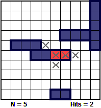
Walkthrough
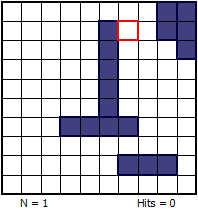
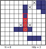
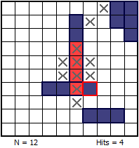
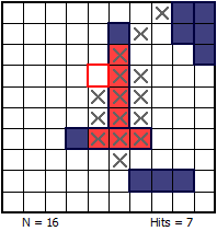
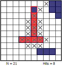
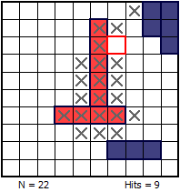
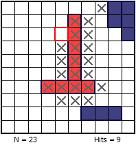
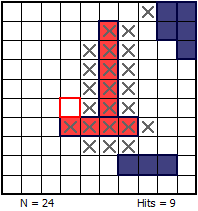
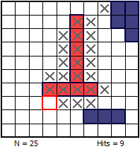
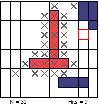
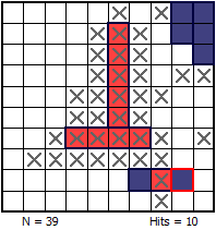
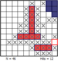
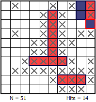
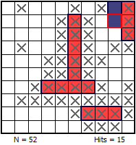
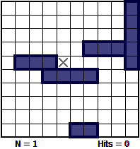
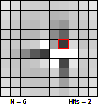
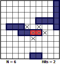
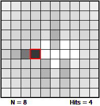
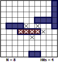
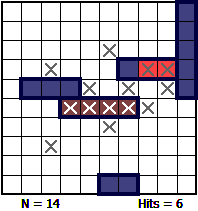
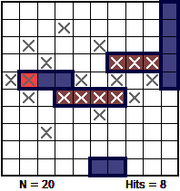
Below is a walkthrough of a sample game using this strategy. The red square shows the target location for the next selected volley.
 |
 |
 |
 |
|
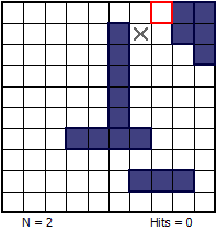
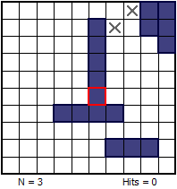
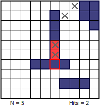
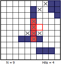
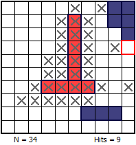
Initially, the algorithm starts in Hunt mode, firing random shots. On turn #3 it has hit something and turns into Target mode. The four cardinal directions (We'll use N, S, E and W to describe direction), are all added to the stack of 'potential' locations as they are touching a know ship location. Going N for turn #4 has resulted in another successful hit, so the locations N, E and W of this new location are added to the 'potential' target stack (S is not added – that location has already been visited!).
|
|||
 |
 |
 |
 |
|
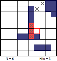
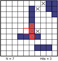
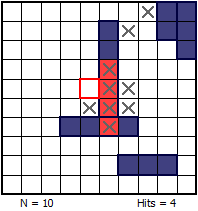
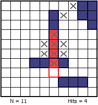
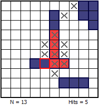
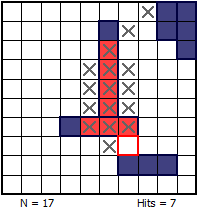
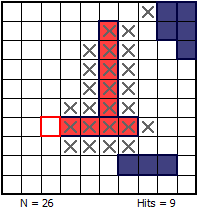
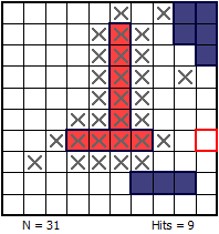
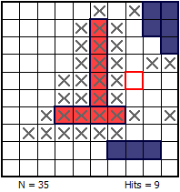
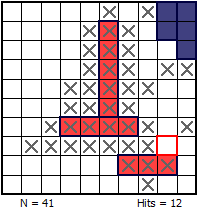
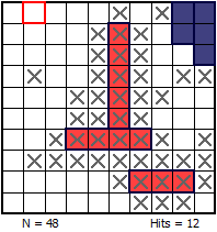
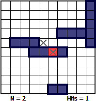
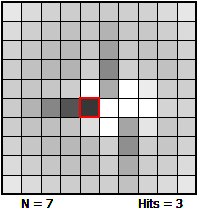
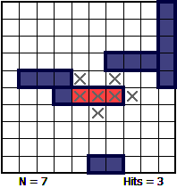
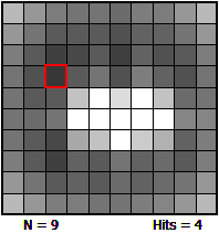
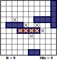
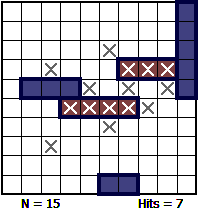
Turn #5 (S of the first hit) is also a hit, so the surrounding squares not already visited are added to the end of the stack. Turn #6 and Turn #7 are misses.
|
|||
 |
 |
 |
 |
|
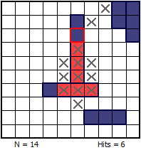
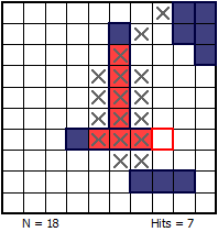
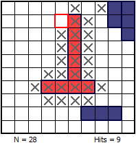
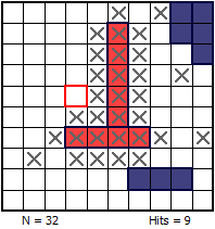
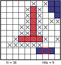
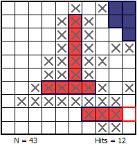
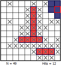
Turn #9 and turn #10 see the computer testing and eliminating squares either side of the target, and turn #12 sees the discovery of a pixel to the side. You can see here why this dumb algorithm needed to perform this test; if it was simply looking for straight lines, it would have stopped searching downwards after the miss on turn #11 and then continued up one more square ontop to sink, what it thought, would be the the aircraft carrier at five units long.
|
|||
 |
 |
 |
 |
|
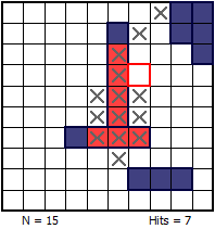
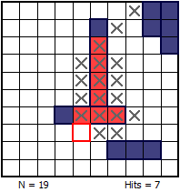
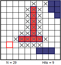
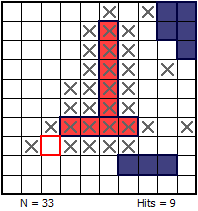
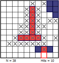
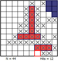
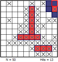
We're now deep into the sinking this ship cluster.
|
|||
 |
 |
 |
 |
|
But, to be sure, we need to visit every touching member around the edge of the a known hit.
|
|||
 |
 |
 |
 |
|
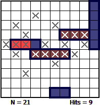
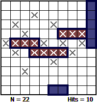
Edge investigation continues, resulting in a new find on turn #21.
|
|||
 |
 |
 |
 |
|
On turn #28, the last 'potential' target is pulled off the stack, drawing a miss. The algorithm will now return to Hunt mode and continue the random search.
|
|||
 |
 |
 |
 |
|
No luck yet …
|
|||
 |
 |
 |
 |
|
Success on turn #36! Returning to Target mode.
|
|||
 |
 |
 |
 |
|
The cruiser has been sunk by turn #40, but the dumb algorithm does not know this, and needs to blindly continue walking around the edge … just to be sure.
|
|||
 |
 |
 |
 |
|
Some of the edges have already been visited by this stage, so searching is faster.
|
|||
 |
 |
 |
 |
|
The miss on turn #45 indicates the end of Target mode and we're back to random Hunt mode.
|
|||
 |
 |
 |
 |
|
We've hit again on turn #49.
|
|||
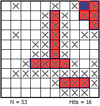 |
The grouping of the final two ships is such that finding the last few squares happens quickly (it's in a corner, so less to add to the stack, and they lay parallel, so share many of the same boundaries). A count is kept of the number of hit pixels, and so on turn #53, when the last salvo brings the count to 17, the algorithm terminates immediately and it does not need to walk around the edges still on the 'potential' stack. |
||
Results
Below is a graph of the results using this basic algorithm on 100 million randomly generated grids.
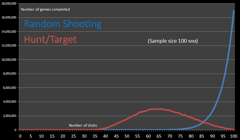
The red line depicts the results of this algorithm and the blue line, for reference, shows the results of pure random guessing. There is an obvious improvement.
Parity
We can make a slight improvement to the Hunt part of the algorithm using parity.
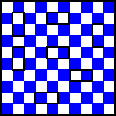
|
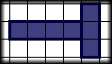
Because the minimum length of a ship is two units long, then we don't need to random search every location on the board. Even the shortest ship has to straddle two adjacent squares. Imagine the board as a checker board, like the grid on the left. No matter how the two unit destroyer is placed on the grid it will cover always cover one white and one blue grid. A mathematical term to describe this is Parity. This is just a fancy word of describing if the square would contain an odd or even number if labelled sequentially from 1 to 100 The blue squares on the grid are even parityand the white squares odd parity. |
|
We can instruct our Hunt algorithm to only randomly fire into unknown locations with even parity. Even if we only ever fire at blue locations, we will at least hit every ship — it's impossible to place any ship so that it does not touch at least one blue square. Once a target as been hit, and Target mode is activated, the 'parity' restriction is lifted enabling all potential targets to be investigated. If the algorithm returns to Hunt mode, again, the parity filter is enabled. (The smarter readers will have realised that, once we've sunk the two unit destroyer, we can change the parity restriction to a larger spacing, and that's the prefect seque into the advanced implementation described further in this article, keep reading …) |
Results
Below is a graph of the results using the modifed parity algorithm.
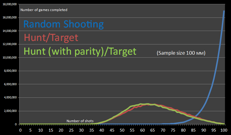
The green line depicts the results of the parity algorithm. The parity algorithm gives improvment over the entire range, but the incremental gain is small. The biggest drain on shots is the unecessary walking around the edges of targets. Using the parity filter in Hunt mode has reduced the shot count, but once the algorithm gets into Target mode, it is just as inefficient as it was. To make futher improvements in strategy, it is this area we need to focus our attention.
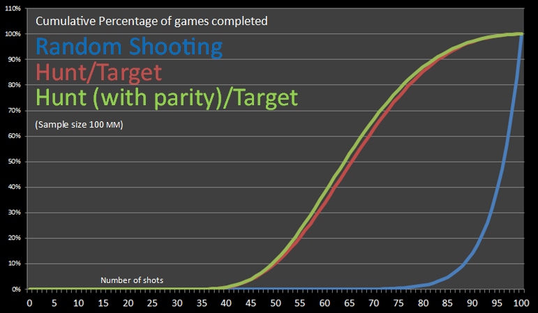
Below is a chart of the cumulative probabilities of finishing the game in n-moves or less, and you can see the improvement of both these basic strategies over pure random guessing.
Full Game Rules
To get more efficient algorithm for solving the game we need to better identify when a ship has been sunk. Thankfully, the official rules of the game help us in this regard. Up until now, we have only used two states for giving feedback on each shot: HIT and MISS.

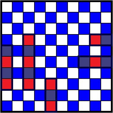
|
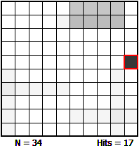
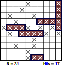
The official rules of the game also state that you should let your opponent know if they have successfully SUNK any ship, so this third style message ”You have sunk my aircraft carrier” conveys much more information than just hit. It tells you the length of the ship you have just hit, it tells you that you have hit all pixels of this ship, and it could, potentially, give you a new minimum size of ship you are searching for (for instance, if you have sunk all ships other than the aircraft carrier, then you know that this remaining ship is five units long and can adjust your random search according to skip the appropriate number of spaced when in hunt mode. In the diagram to the left, SUNK entities are rendered in brown with white crosses. |
Probability Density Functions
Now that we will be told when a ship is sunk, we know which ships (and even more importantly what the lengths of the ships) are still active. These facts are very valuable in determining which location we search next.
Our new algorithm will calculate the most probably location to fire at next based on a superposition of all possible locations the enemy ships could be in.
At the start of every new turn, based on the ships still left in the battle, we’ll work out all possible locations that every ship could fit (horizontally or vertically).
Initially, this will be pretty much anywhere, but as more and more shots are fired, some locations become less likely, and some impossible. Every time it’s possible for a ship to be placed in over a grid location, we’ll increment a counter for that cell. The result will be a superposition of probabilities
 |
"Once you eliminate the impossible, whatever remains, no matter how improbable, must be the truth." Arthur Conan Doyle - Sherlock Holmes |
Examples
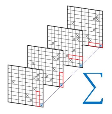
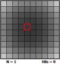
In the following simple examples, we're just looking at the probabilities for the location of an aircraft carrier (length 5 units). We start in the top left corner, and try placing it horizontally. If it fits, we increment a value for each cell it lays over as a 'possible location' in which there could a ship. Then we try sliding it over one square and repeating … and so on until we reach the end of the row. Then we move down a line and repeat. Next we repeat the exercise with the ship oriented vertically.
Sometimes the ship will fit a space, sometimes it will not. As the board becomes more and more congested (with hits, misses and sunk ships), the number of possible positions the ships can fit reduces. It's not the absolute number, however, we're looking for. We're simply looking for the most likely location for a ship to be located in based on the information we already know.
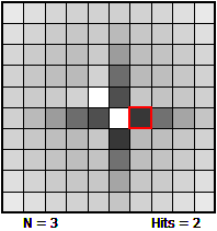
Whilst the examples below show just the probablity distributions for where an aircraft carrier could be hidden, for the full implementation we iterate through each not-yet-sunk ship adding them together to create the superposition. The algorithm selects the location with the highest count of possible ships that could be positioned through that square.
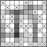
 |
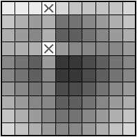
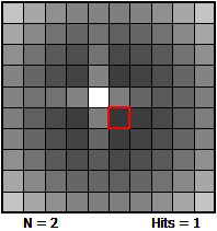
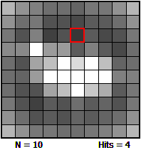
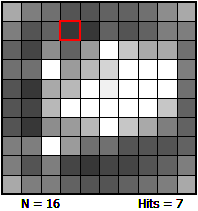
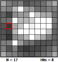
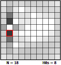
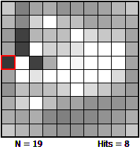
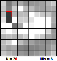
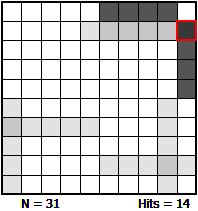
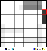
In all these examples, shading is used to depict the probability. Dark colours represent high probabilty, and light colours represent low probability. In this example, one shot has been fired, and we're looking for the aircraft carrier. It's less likely to be South (because it could not fit vertically, and so the only way it could overlap one of the cells to the South is if it layed horizontally). Similarly, it's less likely to be West. Probablities also fall off slightly towards the edges and corners as there are less ways to position the ship that covers these locations. |
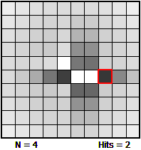
 |
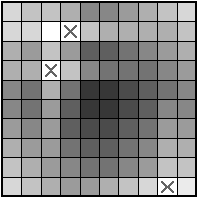
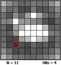
With two misses on the grid, it's less likely to be in the space between the two misses. It's also very unlikely to be on the top row to the left, as here it can only be placed vertically. White squares represent zero probability, and by definition, any square that is a miss has zero probability. |
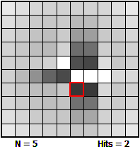
 |
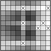
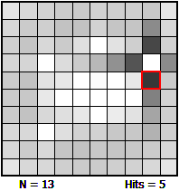
In this configuration we can see a white square just to the left of the top miss. It is impossible for the aircraft carrier to pass through this square. |
 |
An example distribution with seven misses on the grid. |
 |
A ficticious board layout with lots of misses marked. Many of the locations are impossible to host the carrier. The darker the shading, the more possible ways that the carrier could use this square. |
 |
Another example with lots of misses. |
This algorithm still has a hunt mode and target mode, though both operate essentially the same way. When in hunt mode, there are only three states to worry about: unvisited space, Misses and sunk ships. Misses and Sunk ships are treated the same (obstructions that potential ships needed to be placed around). In target mode (where there is at least one hit ship that has not been sunk), then ships can, by definition, pass through this location, and so hit squares are treated as unvisited space squares for deciding if a ship 'could' pass through this square, and then a heavy score weighting is granted to possible locations that pass through a point we know already know contains a hit.
Results
Here are the results of the new algorithm. As you can see, the results are signifincantly better. No game took longer than 73 moves to complete, and approximately one in every million games played with random boards was a perfect game (completed in 17 moves, each a hit and no misses).
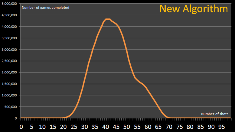
The mediam game length with this algorithm in 42 moves cf. 97 moves with a purely random shooting pattern, and 64 moves with a parity filtered hunt/target algorithm.
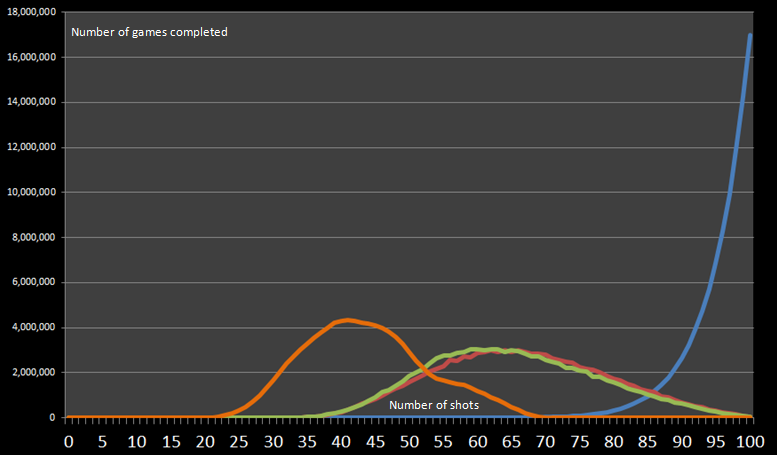
Here are the results of 100 million random games using each algorithm, plotted on the same scale.
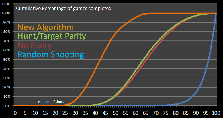
Finally, here is a chart of their cumulative probabilities.
Walkthrough
Here's an example of the algorithm walking through a random board. It solves this puzzle in 34 moves.
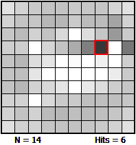
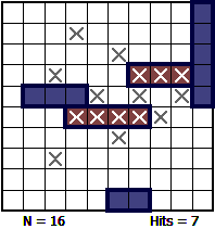
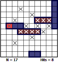
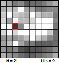
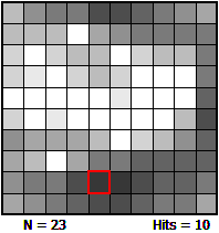
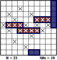
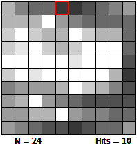
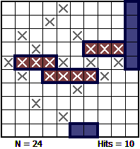
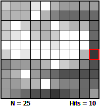
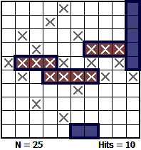
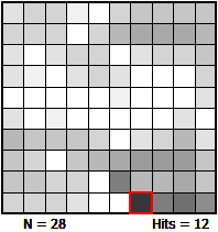
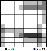
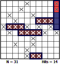
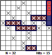
The image on the left shows the probability distribution, and the red-reticle shows the selected next location to fire at. The image on the right shows the current state of the grid.
 |
With no information about the board, the algorithm selects one of the center squares. Because of the edge effect described earlier, the middle of the board will score higher than an edge or a corner. Unfortunately, the first shot ends in a miss |
 |
 |
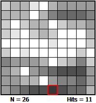
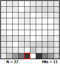
With the knowledge of the first miss, the algorithm recalculates the probability density and selects the current highest scoring sell (or one of them, if there are more than one that share the same value). This time, it's a hit |
 |
 |
The four surrounding squares are all equal in probablity (this being a square close to the center, so still able to host part of an aircraft carrier in all directions), and the cell to the right is chosen. Another hit |
 |
 |
Now that there are two hits in a row, the highest probability targets are to either side of these two. The shot to the right is a miss |
 |
 |
Interestingly, at this point, it's just as likely that the two hits could be from two parallel up/down ships as one side to side, and in this implementation of the alogrithm if there is more than one location with the same probability, the next numeric one (starting from the top-left) is selected. This is also a miss |
 |
 |
Another miss. (Notice that the algoritm tested the top side this time, and the lower side previously, gaining knoweldge becasuse of a parity skip between it and the miss two to the left. |
 |
 |
Now we pretty sure that we need to move left (since we know all ships are still in play), and the chances are very low that the soution is down/up/down ships. |
 |
 |
Success, we've sunk our first ship. Since we receive indication that a ship is sunk, the algorithm does not heavily weight continuing further to the left. It will go there if needed, but based on the probability that another ship is in this space, not as a continuation of the current ship. |
 |
 |
Hunting shot based on the probability of ships being in this location |
 |
 |
More hunting shots. |
 |
 |
And again. |
 |
 |
Another hit. |
 |
 |
Since long ships are still in play, it's slightly more likely that ships run up/down from this location (and slightly more likely down than up, since the aircraft carrier would not fit upwards). |
 |
 |
Miss |
 |
 |
Another ship sunk (and thus removed from the probability cloud). |
 |
 |
Back to hunting. |
 |
 |
Another hit. |
 |
 |
Again, with the big ship still in play, it's slightly more likely that it ships run up/down. |
 |
 |
Miss. |
 |
 |
Miss. But again notice the skipped vertical parity as it tried the vertical space two up, not just one up. |
 |
 |
Hit. |
 |
 |
Another ship sunk. |
 |
 |
Back to hunt mode. |
 |
 |
Checking the larger white spaces. |
 |
 |
 |
|
 |
 |
|
 |
Hit. |
 |
 |
Checking to the side first, as the aircraft carrier is still out there, and can only run left-right from here. |
 |
 |
Success in shrinking the destroyer. This is good fortune for us. The destroyer is length 2, and with this sunk, it only leaves the aircraft carrier, which is large, and harder to hide. With the removal of the destroyer there probability cloud will change considerably. There are not that many loations left where the aircraft carrier can be. |
 |
 |
Large areas of the board are now white. The alogithm starts to search, initially, in the biggest area of possible space (highest probability, since there are many ways that the carrier could lay in this area). |
 |
 |
Hit! It's only a few moves to victory from here. |
 |
 |
 |
|
 |
 |
|
 |
Game Over! |
 |
Thanks for reading.
You can find a complete list of all the articles here. Click here to receive email alerts on new articles.
© 2009-2013 DataGenetics