
	Advertisment

Parrondo's Paradox

“How two ugly parents can make a beautiful baby”

In today’s posting, I’m going to look into Parrondo’s Paradox. It is named after the person who discovered it in 1996, Spanish physicist Juan Parrondo.

Parrondo’s Paradox is one of those counterintuitive puzzles to which your first reaction is going to be “No Way, that can’t possibly be correct!” Next, you’ll probably fire up Excel or Visual Studio and write some code to test it for yourself. Go for it!

We’re going to show how, mathematically, two wrongs can sometimes make a right. Here we go …

The Set-up

Imagine there are two casino games: Game A and Game B.

Each game is random, and each of them has odds stacked against the player (they have a negative expected outcome). Each time either game is played, if you win, you win $1, if you lose, you lose $1.

If you play Game A continuously you’ll gradually lose money. The longer you play, the more money you will lose; not good for your retirement plans!

Similarly, if you play Game B continuously you’ll gradually lose money.

However, what if I told you that if you alternate playing these two games using the pattern: A, B, B, A, B, B, A, B, B, … that the odds will switch to being in your favor ?!?!

Huh? Yes, that’s right! By alternating play you can turn these two loss making games into a money making exercise with a positive expected outcome. This is Parrondo’s Paradox.

Background

Let’s start our investigation with discussion about a neutral game. Imagine we have a totally fair and unbiased coin. This coin lands 50:50 heads/ tails when flipped.

We start off with zero dollars and flip the coin. If it lands heads, we win a dollar. If it lands tails, we lose a dollar. Then we play the game again, and again.

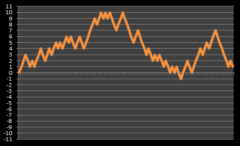
After multiple flips, our balance will jitter up and down, but it should average around the break-even point. To the right is a graph of how our balances might look after a series of consecutive flips. The x-axis shows the number of flips, and the y-axis shows the balance.

This curve is often described as a “Drunken Man’s Walk”

If we repeated this experiment many, many times and averaged the results, then the jitters would be smoothed out. Below is a plot for our fair coin after 1,000,000 parallel experiments of 500 consecutive flips.

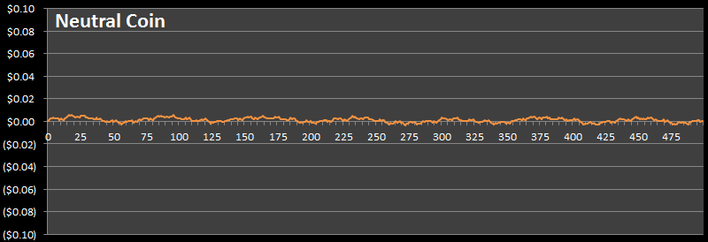
As you can see, it’s pretty flat (note the scale on the left), over a million games, the average never moves more than a fraction of a penny away from zero. This is what we’d expect. The expected outcome of a fair coin is break-even.

Game A

Now we know what a fair coin looks like, let’s create our first losing game: Game A.

Game A is also played with a coin but this time it’s played with an unfair coin, and the bias is against the player.

We’ll define the probability of this bias to be: ε

The chance of winning the biased coin toss Game A = 0.5 - ε

The chance of losing the biased coin toss Game A = 0.5 + ε

For the calculations in this posting, I’m going to use a value of ε = 0.005

So, for Game A, the probability of the coin landing heads is Pr = 0.495 (win), and the probability of it landing tails is Pr = 0.505 (loss).

Over time, it’s clear that we’re going to lose on this game if we play it.

Here is a chart of showing how our balance changes after 500 flips. As before, I’ve averaged the results over a million sets of games.

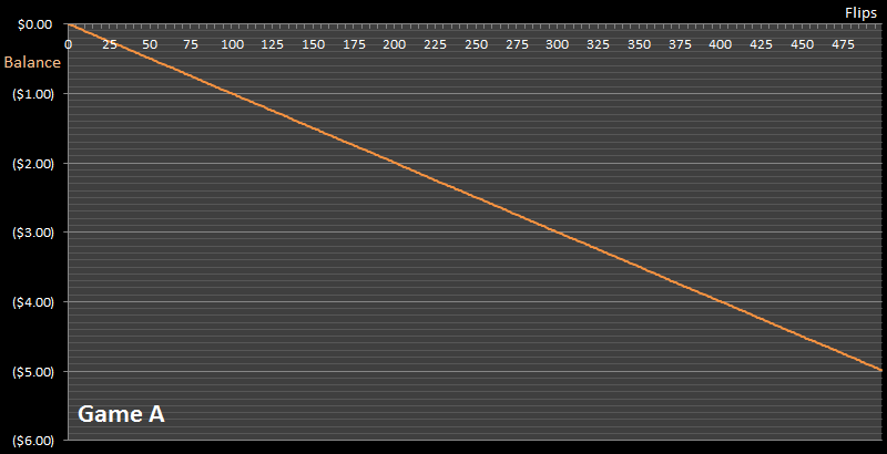
Sure enough, over time we lose money playing this game. You can see the line sloping down to the right.

Modeling this game with lots of random flips is called a Monte-Carlo Simulation, as we can see, at 500 flips, after a million games, our average finishing balance is -$4.998, which is very close to the expected result we get from a Bayesian model approach. Using subjective analysis, after 500 flips, our theortical expected loss should be 500 x ( (0.495 x $1) + (0.505 x $-1) ), which equates to $5.00

Game B

The rules of Game B are a little more complex but it’s also a losing game.

For this game we have two (different) coins we could flip instead of one. To determine which coin to flip, we look at the current value of our cash balance. If the money we have is currently a multiple of three we flip the first coin (Coin B1). If the money in our current balance is not a multiple of three we flip the second coin (Coin B2).

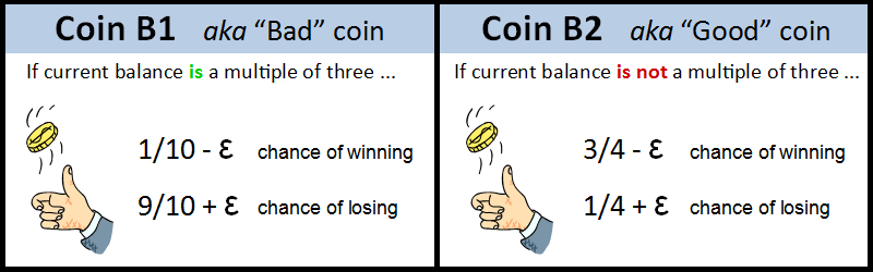
As you can see, the two coins have very different probabilities. Coin B1 (which I’ll call the ‘bad’ coin), is brutal, giving the player a less than 10% chance of winning. Thankfully we only flip this coin if our current cash balance is a multiple of three. Coin B2 (the ‘good’ coin) gives the player just less than 75% chance of winning.

It’s hard to tell just by looking at the formulae, but this game is also losing game. Here’s a plot of the average balance obtained after playing a million sets of games to 500 rounds.

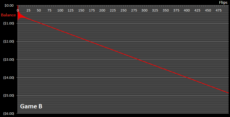
Again the line slopes down to the right. The longer your play, the more money you stand to lose. This game also has a negative expected outcome.

(The oscillations on the left of the curve are explained below).

Mathematical proof for Game B

Warning Math ahead! This section is optional, feel free to skip.

The curve above shows the balance for playing Game B using a Monte-Carlo simulation. How would we go about calculating the exact expected value of this game?

At first glance, you might think that since we take the Modulus 3 of the balance (to find out if the balance is a multiple of three), that the bad coin is flipped 1/3^rd of the time, and the good coin is flipped 2/3^rds of the time. If that is true then the chance of winning would be:

Pr(win) = 1/3 x (1/10 – ε) + 2/3 x (3/4 – ε)

Which, for ε = 0.005, equates to a Pr = 0.5283, which is greater than 50%! This would imply that Game B should be a winning game, not a losing game. Huh? What’s going on? We know from experimentation that balance decreases over time, so it is losing game !?!

I have to admit, when I first modeled at this game, I made the same mistake as above. The true explanation is that the moduli of the current balance do not occur with equal probability!

Let me explain: If the current balance happens to be a multiple of three, you’re going to be flipping the bad coin. It’s much, much more likely that you’ll lose the flip of the bad coin and end up back at a modulus one below your current state. So now you’re in the state of the modulus one before the multiple of three and you’ll be flipping the good coin. There is a higher probability of winning this game, so you’ll end up back at a multiple of three. As you can see, it’s more likely you’ll be oscillating between these states than progressing simply up or down! This adjusts the weightings about how likely you will be in each of the moduli.

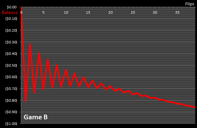You can see this effect early on in the simulation graph. A close-up is shown on the left.

Before the number of flips gets large and things merge into one, you can see the oscillations clearly as the average balance moves between these states.

To work out the exact probabilities we can bring out one of my favorite tools, the Markov Chain. (For more background reading on this, check out my postings about using Markov Chains to solve Chutes and Ladders, Candyland and Yahtzee).

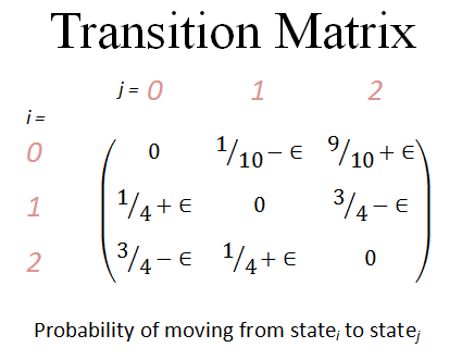
Let’s define the three states of our Markov model to be the Modulus (3) of the current balance (The remainder if we divided the balance by three). It can have the values { 0 , 1 , 2 }

Here is the Transition Matrix showing the probabilities of moving from state_i to state_j

As you can see, each row is stochastic and adds up to 1.0 (something has to happen on each coin flip), and there are zero’s on the leading diagonal (it’s not possible to stay in the same state). Each element of the matrix represents the probability of moving from that modulus state to another.

Setting up our starting conditions, we can multiple our input vector by the transition matrix, then feed these answers back in and multiply again, and again, and again. Here is chart showing how the probabilities of being in any of the modulus states changes over time. As you can see it initially oscillates wildly, but soon asymptotes to a steady state. These are the expected probabilities for being in each state after a large number of flips.

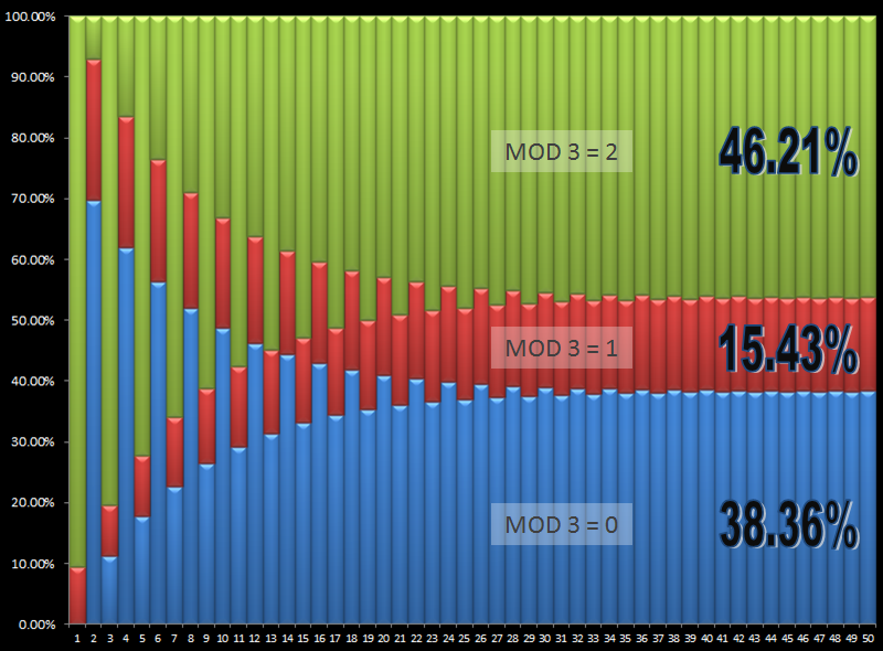
After things settle into steady state, the probability of being in Modulus state zero (flipping the ‘bad’ coin) is 38.36%

The probability of being in Modulus state one or two (flipping the ‘good’ coin) is 61.64% which is (15.43% + 46.21%)

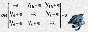We can read these probabilities off the chart, but mathematically, there is another way to determine the answer. We can determine the answer by calculating the Eigenvectors for this matrix (I think I’ve probably lost a good number of people in this post already, so if you’re still reading this, I assume you’re familiar with Eigenvectors).

There are three Eigenvalues for the above matrix. One Eigenvalue is 1.0 representing the steady state for a large number of flips, and the smaller two are complex. (In fact, for all Transition matrices that are stochastic, there should always be a an Eigenvalue which is 1.0 and this corresponds to the steady state).

Back to the Paradox

We’ve now shown how both games, played by themselves, are losing propositions.

Here is a graph of our balance if we play Game A once, followed by Game B twice, then repeat the pattern ABBABB …

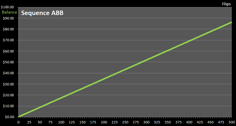
As you can see, the balance line goes up. Over time, with this combination of games, we can make money. This is Parrondo’s Paradox. We’ve turned two losing games into a winning game.

Different combinations of sequences of A and B produce different results. Some combinations create money making games, some combinations do not.

So what’s going on?

The key to understanding this paradox is that the two games are not independent.

Recalling back to the Markov Analysis of Game B, we learned that probability distribution for the moduli of the cash balance is not uniform. Alternating the games allows the system to more likely get into a state in which the ‘good’ coin is flipped, and this particular coin is biased in favor of the player. The combination of games allows the system to ratchet up winnings.

(For instance, it’s not hard to imagine the system getting in the state where a flip of the almost-even coin wins (great), but even in a loss, it puts the player back into a state where the next coin flipped is the ‘good’ coin again, with much stronger odds of getting the player back to where they just were).

Other examples

If you’ve read my article on Chutes and Ladders you may recall in the last section I explained the seemingly paradoxical situation where it is possible to add additional chutes to a game board and reduce the average length of a game! How come? Well, if you have a long ladder in the game (such that landing on one will propel you far up the board for a strong advantage), and you miss it; If the added additional chutes on the board send you back to before this long ladder, then you have a second attempt to hit the long ladder!

A second (or third …) attempt at the long ladder is potentially much more benefecial to you than the backtacking the additional chute caused you.

Have you ever shaken a tin of mixed nuts? If you have, you would have found out that, paradoxically, the larger and heavier nuts ‘float’ to the surface (against a gravity gradient), and the smaller, lighter, nuts sink to the bottom. What’s going on?

Well, the smaller nuts are able to find the small gaps and imperfections in the nesting of the nuts and work their way down the tin with the shaking. The larger nuts are not able get through the gaps. This phenomenon is given lots of fun names. Physicists describe it as Granular Convection, but I’ve also heard it called the Museli effect (since it often happens to breakfast cereals in shipment), and yes, it’s sometimes called the Brazil nut effect.

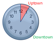
Another classic example is the Martin Gardner puzzle about the man with two girlfriends and the subway station. (Martin Gardner was my favorite author growing up. You can read my a tribute blog posting to him here).

In this puzzle, a man has two girlfriends, both of whom he likes equally. One lives uptown, and the other downtown. He decides to let chance determine which lady he visits each day, so he arrives at the subway station at a random time, stands on the platform, and then takes the first train that arrives.

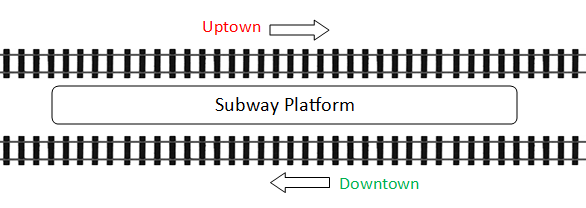The same number of trains travel uptown as downtown, and though he arrives at the station at a totally random time each day, he finds out that he is visiting the girl downtown over ten times as often as the girl uptown. What’s going on?

The solution is that, even though the trains arrive with the same frequency, the uptown train departs just a few minutes after the downtown train has departed. Because of this, there is only a narrow time window in which the man is able to get on the uptown train.

If they married, and had children, do you think they would be beautiful?

You can find a complete list of all the articles here. Click here to receive email alerts on new articles.